Income and Substitution Effects of a Price Change

The Total, Substitution, and Income Effects

When the price of a good changes, the consumer moves from an initial optimal bundle (let's call it A) to a new final bundle (let's call it B). The overall change in consumption from A to B is the total effect. Our task is to decompose this total effect into two conceptual parts:

1. The Substitution Effect (SE): This captures the change in consumption due solely to the change in relative prices. We isolate this by imagining the consumer stays on their original indifference curve (maintaining the original level of utility) but faces the new price ratio. They will substitute away from the good that has become relatively more expensive. For a price increase, the substitution effect is always negative.

2. The Income Effect (IE): This captures the change in consumption due solely to the change in purchasing power or "real income." A price increase makes the consumer effectively poorer, while a price decrease makes them richer. This is equivalent to the type of income change we studied in the last lesson—a shift from one budget line to a parallel one. The direction of this effect depends on whether the good is normal or inferior.

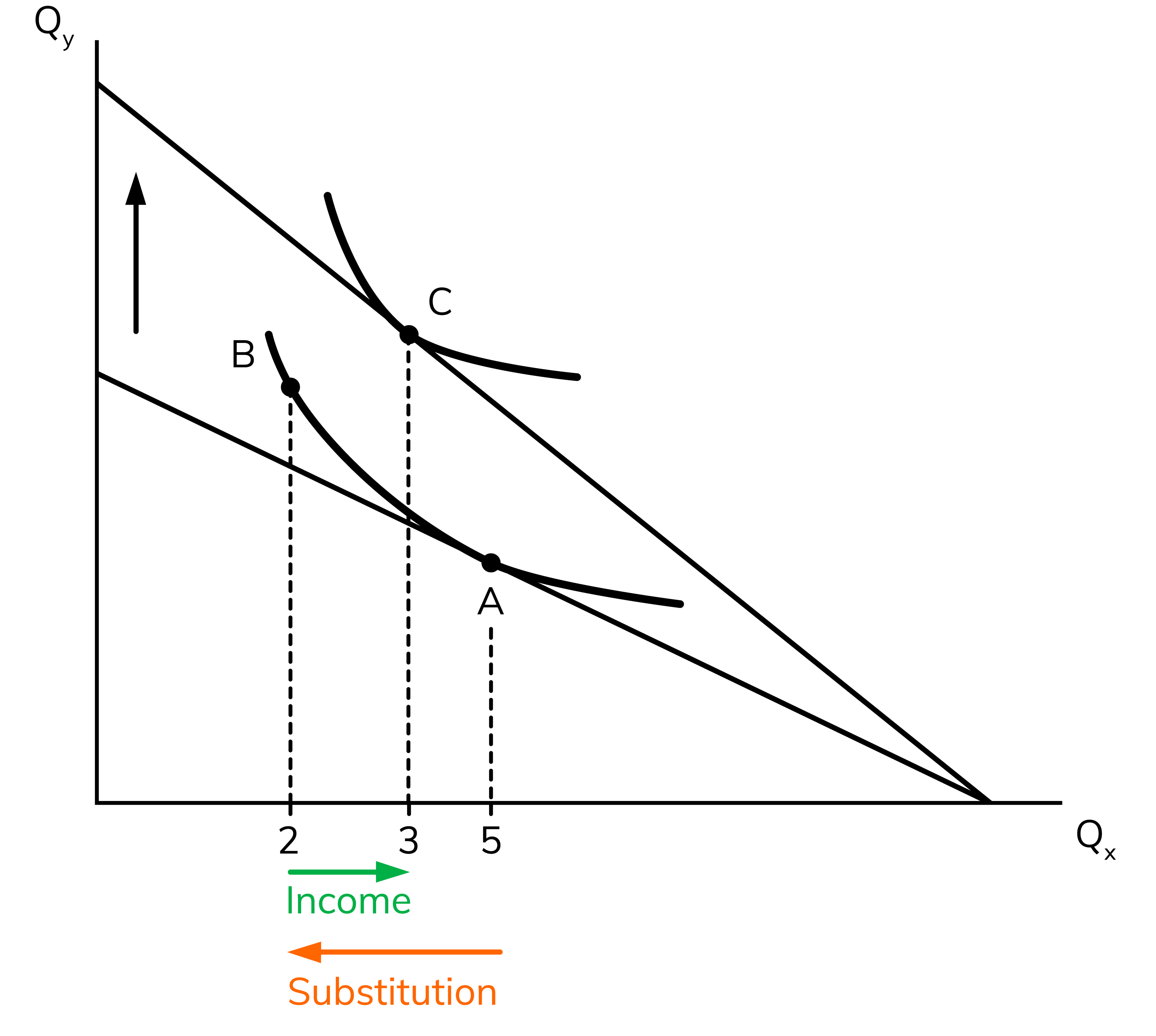
The following diagram illustrates a price increase for good X. The initial bundle is A. The final bundle is B. The total effect is the move from A to B. We introduce a hypothetical intermediate bundle, C, which lies on the original indifference curve but is tangent to a budget line with the new slope.

• The move from A to C is the substitution effect.
• The move from C to B is the income effect.

Calculating the Income and Substitution Effects (Hicksian Decomposition)

Your preference for formal problem-solving will be well-served here. The process, known as Hicksian decomposition (after economist John Hicks), involves three utility maximization problems.

Let's assume the price of good X, $P_X$, increases.

Step 1: Find the initial optimal bundle (A).
Solve the standard utility maximization problem with the original prices ($P_X,P_Y$) and income ($I$).

• Condition 1: $MRS=M{U}_X/M{U}_Y=P_X/P_Y$
• Condition 2: $P_{X}X+P_{Y}Y=I$
  This gives you the bundle $(X_A,Y_A)$ and the initial utility level, $U_A=U(X_A,Y_A)$.

Step 2: Find the final optimal bundle (B).
Solve the utility maximization problem again, but with the new price of good X, $P_X^{\prime }$.

• Condition 1: $MRS=M{U}_X/M{U}_Y=P_X^{\prime }/P_Y$
• Condition 2: $P_X^{\prime }X+P_{Y}Y=I$
  This gives you the final bundle $(X_B,Y_B)$.

Step 3: Find the hypothetical intermediate bundle (C).
This is the key step. We need to find the bundle $(X_C,Y_C)$ that the consumer would choose if they faced the new prices but were "compensated" to remain on their original utility level.

• Condition 1: $MRS=M{U}_X/M{U}_Y=P_X^{\prime }/P_Y$ (reflecting new relative prices)
• Condition 2: $U(X,Y)=U_A$ (reflecting original utility level)
  Solving this system of two equations gives you the intermediate bundle $(X_C,Y_C)$.

Step 4: Decompose the total effect.

• Total Effect = $X_B-X_A$
• Substitution Effect = $X_C-X_A$
• Income Effect = $X_B-X_C$
  You can verify that Total Effect = Substitution Effect + Income Effect.

The following video provides a complete, worked-out example of this entire process. It uses a Cobb-Douglas utility function, which should be familiar from our previous lessons.

Linking the Decomposition to Types of Goods

The power of this decomposition is that it explains why a demand curve might have a certain shape.

• Substitution Effect: As noted, this is always negative for a price increase and positive for a price decrease. When relative prices change, a rational consumer always substitutes towards the relatively cheaper good. This is a robust theoretical result.

• Income Effect: This depends on the nature of the good, which we analyzed last lesson.

  • For a normal good, a price increase (which reduces real income) causes consumption to fall. The income effect is negative ($IE<0$).
  • For an inferior good, a price increase (reducing real income) causes consumption to rise. The income effect is positive ($IE>0$).

This leads to three possibilities for the total effect of a price increase:

1. Normal Good: $SE<0$ and $IE<0$. The two effects reinforce each other. The total effect is unambiguously negative. The law of demand holds.
2. Inferior Good (non-Giffen): $SE<0$ and $IE>0$, but $|SE|>|IE|$. The substitution effect, which pushes consumption down, outweighs the income effect, which pushes it up. The total effect is still negative. The law of demand holds.
3. Giffen Good: $SE<0$ and $IE>0$, but $|SE|<|IE|$. The good is so strongly inferior that the positive income effect overwhelms the negative substitution effect. The total effect is positive. A price increase leads to an increase in quantity demanded, violating the law of demand. These are rare in practice but theoretically important.

The following reading provides a rigorous explanation for why the substitution effect is always negative and formally introduces the Slutsky equation, which you might find interesting as it relates the change in demand to these components using derivatives.

An Alternative Method: The Slutsky Decomposition

For completeness, it's worth knowing there is a slightly different but equally valid method proposed by economist Eugen Slutsky. The only difference is in how the "intermediate" bundle is calculated (Step 3).

Instead of finding a bundle on the original indifference curve, the Slutsky method calculates the income needed to afford the original bundle (A) at the new prices. This "Slutsky compensation" is a tangible amount of money, making it popular for empirical studies.

The steps are the same, but the calculation for the intermediate bundle is different. The video below provides a clear, numerical example. Given your background, you may appreciate this alternative quantitative approach.

For most purposes, especially within the scope of the CB2 exam, the Hicksian method is standard. However, knowing that an alternative exists based on a different definition of constant "real income" adds depth to your understanding.

Conclusion

This lesson has provided the analytical tools to dissect a consumer's response to a price change. We have moved beyond simply observing that consumption changes and can now explain precisely why it changes, attributing the shift to the distinct forces of substitution and income.

Key Takeaways:

• The total effect of a price change can be decomposed into a substitution effect and an income effect.
• The substitution effect captures the response to a change in relative prices, holding utility constant. It is always negative for a price increase.
• The income effect captures the response to a change in purchasing power. Its sign depends on whether the good is normal (IE reinforces SE) or inferior (IE opposes SE).
• The sum of these two effects determines the total change in quantity demanded and explains the slope of the demand curve. In the rare case of a Giffen good, a strong positive income effect outweighs the negative substitution effect.

With this lesson, we conclude our deep dive into consumer theory. You are now equipped to model and predict consumer behavior in response to changes in their economic environment. In our next module, we will pivot to the other side of the market and begin our study of the theory of the firm, starting with the fundamentals of production.