Measuring Productivity: Total, Average, and Marginal Product

Introduction

In the previous module, we completed our study of consumer theory, culminating in a method to decompose how a consumer responds to a price change. We now pivot from the demand side of the market to the supply side. To understand why firms make the supply decisions they do, we must first look "under the hood" at the process of production itself.

This lesson begins our exploration of the theory of the firm by focusing on the fundamental relationship between inputs and outputs. Our goal is to calculate three key metrics that describe a firm's productivity: total product, average product, and marginal product. Mastering these calculations is the first step toward understanding a firm's costs and, ultimately, its profit-maximizing decisions.

From Inputs to Outputs: The Production Function

At its core, a firm exists to transform inputs into outputs. The inputs, also known as factors of production, are typically categorized as land, labor, capital, and entrepreneurship. The output is the good or service the firm sells. The technological relationship that specifies the maximum output that can be produced with any given combination of inputs is called the production function.

In the short run, we assume at least one input is fixed (e.g., the size of a factory or the number of sewing machines in a workshop). Other inputs, like labor, are variable. Our focus today is on how output changes as we vary a single input, holding all others constant.

To analyze this, we use three related concepts:

Total Product (TP): The total quantity of output produced with a given amount of the variable input.
Marginal Product (MP): The additional output generated by using one more unit of the variable input.
Average Product (AP): The output per unit of the variable input.

The following reading from the "ECON 150: Microeconomics" text provides an intuitive introduction to these ideas using a simple widget-making example. It also introduces the crucial concept of diminishing returns, which we will explore further in our next lesson.

ECON 150: Microeconomics

This text introduces the core concepts of production in the short run. It explains why productivity might first increase due to specialization before eventually decreasing.

Please read the sections titled Marginal Product and Diminishing Returns. As you read, focus on: The definitions of Total Product and Marginal Product. The idea of specialization leading to an initial increase in marginal product. The Law of Diminishing Marginal Returns and why it occurs (e.g., scarcity of the fixed input). The excellent analogy comparing the relationship between marginal and average product to your semester and cumulative GPA.

Calculating Production Metrics from Data

For your CB2 exam, you will frequently be asked to calculate these metrics from a table of production data. The formulas are straightforward:

Let $L$ be the units of the variable input (e.g., labor) and $T P$ be the total product.

Average Product of Labor ( $A P_{L}$ ):
$A P_{L} = \frac{T P}{L}$
Marginal Product of Labor ( $M P_{L}$ ):
$M P_{L} = \frac{Δ T P}{Δ L}$
Where $Δ$ denotes "change in". If the change in labor is one unit at a time, this simplifies to the change in total product from one worker to the next.

Let's look at a completed example. The table below shows the calculations for each metric as the "Variable Factor" (e.g., workers) increases from 1 to 7.

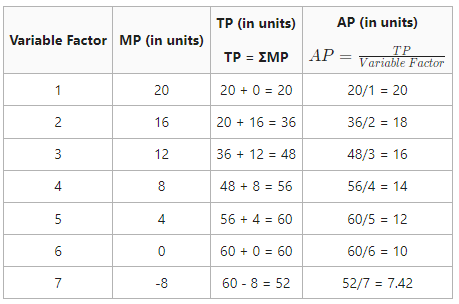
This table illustrates the calculation of Total Product (TP), and Average Product (AP) from given Marginal Product (MP) data. Notice that TP is the cumulative sum of MP, and AP is TP divided by the number of variable factors.

For instance, when moving from 2 to 3 workers:

The MP of the 3rd worker is 12.
The TP becomes the previous TP (36) plus the new MP (12), so $36 + 12 = 48$ .
The AP is the new TP (48) divided by the number of workers (3), so $48/3 = 16$ .

Now, let's work through a problem where you need to find the missing values yourself. This is a very common exam format. The following video provides a step-by-step guide to solving this type of table problem.

Table Problem: Solving for Total Product, Marginal Product, and Average Product

The video "Table Problem: Solving for Total Product, Marginal Product, and Average Product" from the channel Economics in Many Lessons is an excellent tutorial for this skill.

Watch the video from the beginning to the end. The presenter will fill in a table with missing values for Total Product, Marginal Product, and Average Product, explaining how to use the formulas to work both forwards and backwards to find the unknowns.

From Discrete Data to a Continuous Function

While tables are useful for exam questions, in economic modeling, production is often represented by a continuous mathematical function. Given your background in statistics, you'll recognize this as moving from a discrete sample to a continuous model.

For a production function, say $Q = f (L, K)$ , where $Q$ is output, $L$ is labor, and $K$ is capital (held fixed), the marginal product of labor is no longer just the change from one unit to the next. It becomes the instantaneous rate of change, which is the partial derivative of the production function with respect to labor.

Marginal Product of Labor: $M P_{L} = \frac{\partial Q}{\partial L}$
Average Product of Labor: $A P_{L} = \frac{Q}{L} = \frac{f ( L , K )}{L}$

A common functional form used in economics is the Cobb-Douglas production function, e.g., $Q = A L^{α} K^{β}$ . The video below demonstrates how to calculate the marginal product of labor (MPL) and capital (MPK) from such a function using partial differentiation. For this lesson's objective, please focus on the calculation of MPL.

finding MPL and MPK from Cobb Douglas Production function

This video, "finding MPL and MPK from Cobb Douglas Production function" by ECON MATHS, provides a clear mathematical derivation.

Please watch the first part of the video, which focuses on deriving the marginal product of labor, from the start of the calculation to the final MPL expression. This will solidify the link between the discrete calculations in the table and their formal basis in calculus.

This mathematical approach provides a more powerful and general way to analyze production, which will become increasingly important as we build more complex models of the firm.

Conclusion

In this lesson, we have laid the groundwork for analyzing firm behavior by focusing on the production process. We have defined and, most importantly, calculated the three critical measures of productivity: total product, average product, and marginal product.

Key Takeaways:

Total Product (TP) is the overall output.
Average Product (AP) measures productivity per worker ( $T P / L$ ).
Marginal Product (MP) measures the contribution of the last worker hired ( $Δ T P /Δ L$ ).
These metrics can be calculated from discrete data in a table, a common task in economics problems.
In a continuous model, Marginal Product is the partial derivative of the production function with respect to the variable input ( $\partial Q / \partial L$ ).

You are now able to quantify a firm's production capabilities in the short run. In our next lesson, we will look more closely at the shape of these product curves, formally analyzing the Law of Diminishing Marginal Returns and showing how it directly leads to the shape of a firm's cost curves.

Recommended resources

Introduction

From Inputs to Outputs: The Production Function

Calculating Production Metrics from Data

From Discrete Data to a Continuous Function

Conclusion