Diminishing Returns and Rising Marginal Costs

The Law of Diminishing Marginal Returns

As we briefly touched upon, when a firm adds more and more of a variable input (like labor) to a fixed input (like capital), the marginal product of the variable input will eventually decline. This is the Law of Diminishing Marginal Returns.

Initially, adding workers might lead to increasing marginal product due to specialization and more efficient use of the fixed capital. However, a point is always reached where the fixed input becomes a constraint. A kitchen with too many chefs or a factory floor with too many workers leads to congestion, and each additional worker contributes less to total output than the one before.

This principle is so fundamental that it dictates the shape of a firm's short-run cost curves. To understand why, we first need to establish the mathematical relationship between marginal product (MP) and marginal cost (MC).

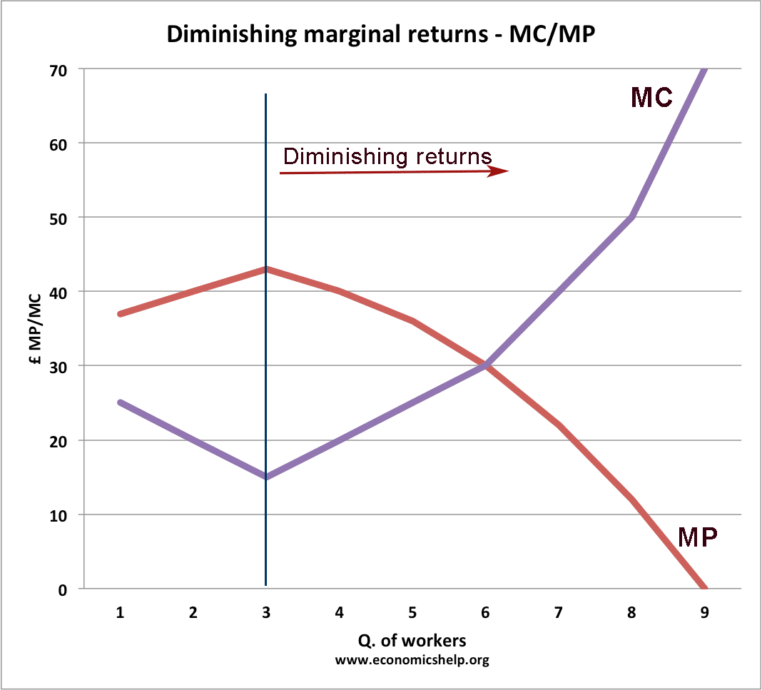
This mirror-image relationship is not a coincidence. Let's derive it from first principles.

The Mathematical Link: From Productivity to Cost

Your background in quantitative analysis will be useful here as we derive the precise relationship between how productive a worker is and how much it costs to produce one more unit of output.

Let's summarize the key steps from the video.

1. Marginal Cost (MC) is the change in total cost ($\Delta TC$) divided by the change in quantity ($\Delta Q$). Since fixed costs don't change with output, any change in total cost in the short run must come from a change in total variable cost ($\Delta TVC$).

   $$MC=\frac{\Delta TC}{\Delta Q}=\frac{\Delta TVC}{\Delta Q}$$

2. Total Variable Cost (TVC) in our simple model is the cost of labor. This is the wage rate ($W$) multiplied by the number of labor units ($L$).

   $$TVC=W\cdot L$$

   Therefore, the change in variable cost is $\Delta TVC=W\cdot \Delta L$ (assuming the wage rate $W$ is constant).

3. Substituting this into the MC formula gives:

   $$MC=\frac{W\cdot \Delta L}{\Delta Q}$$

4. We can rewrite this as:

   $$MC=W\cdot \left(\frac{\Delta L}{\Delta Q}\right)$$

5. Finally, recall from our last lesson that Marginal Product of Labor ($M{P}_L$) is $\frac{\Delta Q}{\Delta L}$. This means that $\frac{\Delta L}{\Delta Q}$ is simply the reciprocal of marginal product, $1/M{P}_L$.

Substituting this final piece gives us the fundamental relationship:

This elegant formula contains a powerful economic intuition:

• When marginal product ($M{P}_L$) is high, each worker is highly productive, adding a lot of output. This means the labor cost embedded in each of those extra units is low, so marginal cost ($MC$) is low.
• When marginal product ($M{P}_L$) is low (i.e., when diminishing returns have set in), each additional worker adds very little to output. To get one more unit of output, you need a larger fraction of an additional worker's time and wage. Therefore, the marginal cost ($MC$) of that unit is high.

A Numerical Demonstration

Let's now apply this formula and observe the relationship using a concrete numerical example.

The video confirms exactly what our formula predicts: as marginal product falls due to diminishing returns, marginal cost must rise.

Practice Calculation

Now, it's your turn to perform the calculation. The image below shows a typical problem you might encounter. A producer, "Shiny Sleeve's," has a production schedule and a fixed wage rate. Your task is to calculate the marginal product and marginal cost.

Let's fill in this table together. Remember the formulas:

• Marginal Product ($MP$) = $\Delta \text{Output}/\Delta \text{Workers}$
• Marginal Cost ($MC$) = $\Delta \text{Total Wage Cost}/\Delta \text{Output}$ which is equivalent to $W/MP$ if the change in input is one unit. Here, since the change in workers is not one, it's safer to use the first formula: $MC=\frac{W\cdot \Delta L}{\Delta Q}$.

Step 1: From 0 to 20 workers

• $\Delta L=20$ workers
• $\Delta Q=80$ units
• Marginal Product: $MP=80/20=4$ units per worker.
• $\Delta \text{Total Wage Cost}=20\text{ workers}\times \$25/\text{hour}=\$500$
• Marginal Cost: $MC=\$500/80\text{ units}=\$6.25$ per unit.

Step 2: From 20 to 40 workers

• $\Delta L=20$ workers
• $\Delta Q=140-80=60$ units
• Marginal Product: $MP=60/20=3$ units per worker.
• $\Delta \text{Total Wage Cost}=20\text{ workers}\times \$25/\text{hour}=\$500$
• Marginal Cost: $MC=\$500/60\text{ units}\approx \$8.33$ per unit.

Step 3: From 40 to 60 workers

• $\Delta L=20$ workers
• $\Delta Q=180-140=40$ units
• Marginal Product: $MP=40/20=2$ units per worker.
• $\Delta \text{Total Wage Cost}=20\text{ workers}\times \$25/\text{hour}=\$500$
• Marginal Cost: $MC=\$500/40\text{ units}=\$12.50$ per unit.

Notice the pattern: as the marginal product falls from 4 to 3 to 2, the marginal cost rises from $6.25 to $8.33 to $12.50. This is a direct numerical confirmation of the law of diminishing returns leading to increasing marginal costs.

Further Practice

To solidify your understanding, work through a couple of problems from the following workbook. This will give you more practice in identifying diminishing returns and linking production data to costs.

Conclusion

In this lesson, we have moved from simply identifying patterns in production to explaining their economic consequences. We established the crucial inverse relationship between marginal product and marginal cost, both through a formal derivation and a numerical example.

Key Takeaways:

• The Law of Diminishing Marginal Returns states that as you add more of a variable input to a fixed input, the marginal product of the variable input will eventually fall.
• This law is the reason for rising short-run marginal costs.
• The mathematical link is given by the formula $MC=W/M{P}_L$, where $W$ is the wage rate.
• As marginal product ($M{P}_L$) decreases, marginal cost ($MC$) must increase.

You are now equipped to understand not just how firms produce, but also the fundamental driver of their short-run cost structure. In our next lesson, we will build on this foundation to construct and analyze the full set of a firm's short-run cost curves: average total cost, average variable cost, and average fixed cost, showing how they all relate back to the marginal cost curve we've explored today.