Introduction
In our previous lesson, we established the fundamental link between a firm's productivity and its costs, deriving the crucial relationship between marginal product and marginal cost (). We saw how the law of diminishing marginal returns is directly responsible for causing marginal costs to eventually rise.
Today, we will expand our view from marginal cost alone to the entire family of short-run cost measures. Your objective is to become proficient in calculating a firm's total cost, average total cost, average variable cost, average fixed cost, and marginal cost from a given set of data. Mastering these calculations is the bedrock for analyzing a firm's profit-maximizing decisions, which we will tackle in upcoming lessons.
The Seven Measures of Short-Run Cost
To analyze a firm's cost structure, we use a set of seven interrelated measures. Let's begin by formally defining them. These definitions are standard across microeconomics and provide the toolkit for our calculations.
Module 9: Cost Curves – Intermediate Microeconomics
This reading from SaskoEr's "Intermediate Microeconomics" text provides concise definitions and formulas for the seven key short-run cost measures.
Please read the section titled "The Seven Short-Run Cost Measures", from the beginning of the section down to the formulas for marginal cost. Pay close attention to the distinction between fixed and variable costs, and how the three average cost measures are derived.
To summarize and organize the key formulas from the reading:
- Fundamental Identity: Total Cost () is the sum of Fixed Cost () and Variable Cost ().
- Average Costs: These are "per-unit" measures.
- Average Fixed Cost ():
- Average Variable Cost ():
- Average Total Cost (): . It also follows that .
- Marginal Cost (): The cost of producing one more unit. Note that marginal cost is the change in variable cost, as fixed costs do not change with output.
Calculating Costs from a Data Table
With these formulas in hand, our primary task is to apply them to a set of production data. A common exam-style problem involves being given a partially filled table and being asked to complete it. The key is to use the relationships between the cost measures to find the missing values systematically.
The following video provides an excellent, step-by-step demonstration of how to tackle such a problem. You'll see how to identify the fixed cost and then use it as an anchor to calculate all other values, sometimes even working backward from an average or marginal cost.
Intro Econ: Completing a Production Cost Table
The video "Intro Econ: Completing a Production Cost Table" by Matt Birch is a practical guide to filling in a standard cost table.
Please watch the video from the beginning to the end. The presenter will first review the formulas and then work through a table row by row. As you watch, focus on the logic used to find each new piece of information: How to identify fixed cost when output (Q) is zero. Calculating MC and the averages for the first unit. Working backward from Average Total Cost to find Total Cost. Working forward from Marginal Cost to find the new Total Cost.
This procedural approach—identifying fixed cost first, then calculating total costs, and finally deriving the averages and marginals—is a reliable method for any such problem.
From Discrete Data to Continuous Functions
Given your background in statistics, you'll appreciate that we can also represent these cost relationships using continuous functions. This approach is more powerful for formal modeling. A firm's total cost can often be expressed as a polynomial function of its output, Q.
For example, a firm might have a total cost function like:
From this single function, we can derive all other cost measures:
- Fixed Cost (FC): The part of the cost that doesn't depend on Q. It is simply the constant term.
- Variable Cost (VC): The part of the cost that does depend on Q.
- Average Costs: Divide the relevant cost function by Q.
- Marginal Cost (MC): The derivative of the total cost function with respect to Q.
The next video demonstrates this process with a different example, reinforcing how to derive each cost function from the total cost function.
deriving total fixed cost total variable cost average cost & marginal cost from total cost function
The video "deriving total fixed cost..." from ECON MATHS shows how to find all cost functions from a given polynomial total cost function.
Watch the entire video from the beginning to the end. It will guide you through: Separating the total cost function into its fixed and variable components. Deriving the average cost functions by dividing by output (X in the video, which is the same as our Q). Finding the marginal cost function by taking the derivative.
Practice Exercise
Now it's your turn to apply these calculation skills. The following exercise is a classic table-filling problem. Use the formulas and the methods from the videos to complete the table.
6.E: Production and Cost Structure of the Firm (Exercises)
This resource from LibreTexts SocialSci provides practice problems on cost structures. We will focus on the first self-check question.
Navigate to the section "7.2: The Structure of Costs in the Short Run". Find the table in Self-Check Question Q1 for the "WipeOut Ski Company". Your task is to fill in the blank columns for Total Cost, Average Variable Cost, Average Total Cost, and Marginal Cost. Instructions: Start by calculating the Total Cost (TC) for each quantity level using the identity TC = FC + VC. The fixed cost is given as $30. Next, calculate the Marginal Cost (MC) for each additional unit produced. Remember, MC = \Delta TC / \Delta Q. Finally, calculate the Average Variable Cost (AVC) and Average Total Cost (ATC) for each quantity level (except Q=0). Once you have completed the table, you can check your work against the provided solution, S1, at the bottom of the section.
From Numbers to Shapes
As a final step, let's connect the numbers we've been calculating to the graphical representation of cost curves. The table and graph below show data for a jacket manufacturer.
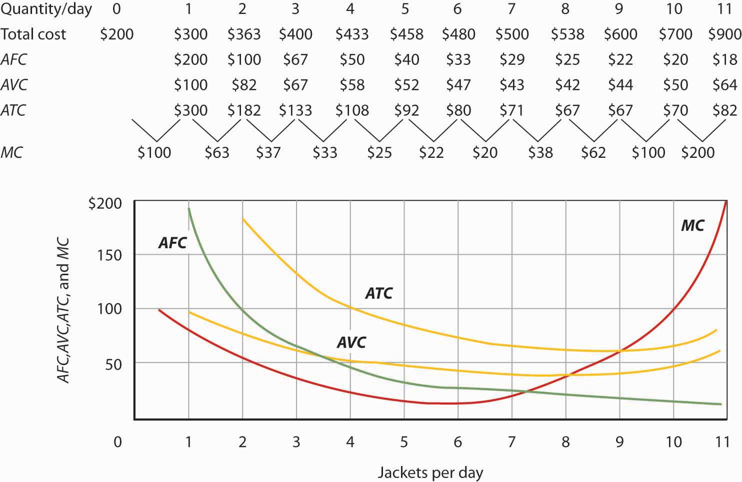
Take a moment to trace a few points from the table to the graph. For example:
- At Q=7, the table shows , , and . Find Q=7 on the horizontal axis and see how these values correspond to the heights of the red (MC), yellow (AVC), and green (ATC) curves.
- Notice that the MC value of $20 at Q=7 is the lowest point on the MC curve before it starts to rise. This corresponds to the point of maximum marginal product, beyond which diminishing returns cause marginal costs to increase.
This visual link between the calculations and the curves is what we will explore in detail in our next lesson.
Conclusion
In this lesson, we have defined and, most importantly, calculated the full suite of a firm's short-run costs. You have practiced these calculations with both discrete data in tables and with continuous cost functions.
Key Takeaways:
- A firm's costs are broken down into fixed costs (unchanging with output) and variable costs (changing with output).
- The seven essential cost measures are C, FC, VC, AC, AFC, AVC, and MC.
- Given any one of Total Cost, Variable Cost, or a set of averages, you can systematically derive all other cost measures using their defined formulas.
- Cost relationships can be analyzed using discrete data tables or continuous functions, with marginal cost being the derivative of the total cost function.
In our next lesson, we will shift our focus from calculation to interpretation. We will plot these cost curves and analyze their characteristic shapes and interrelationships, such as why the marginal cost curve always intersects the average total cost and average variable cost curves at their minimum points.