Graphing Short-Run Cost Curves

Introduction

In our last session, we focused on the mechanics of calculating the seven essential short-run cost measures. You learned to derive everything from fixed and variable costs to the various averages and, crucially, marginal cost, using both data tables and continuous functions.

Today, we transition from calculation to interpretation. Our goal is to visualize these costs by plotting them and, most importantly, to understand the geometric and mathematical relationships between them. You will learn to plot the standard short-run cost curves and, critically, verify why the marginal cost (MC) curve must intersect the average variable cost (AVC) and average total cost (ATC) curves at their precise minimum points. This graphical insight is fundamental for our upcoming analysis of how firms decide their profit-maximizing level of output.

From Data to Curves: The Characteristic Shapes

In the previous lesson, you practiced filling out cost tables. The end result of such an exercise is a set of data points, like the table shown in the top half of the image below. The real power of this data is unlocked when we plot it to create cost curves, as shown in the bottom half.

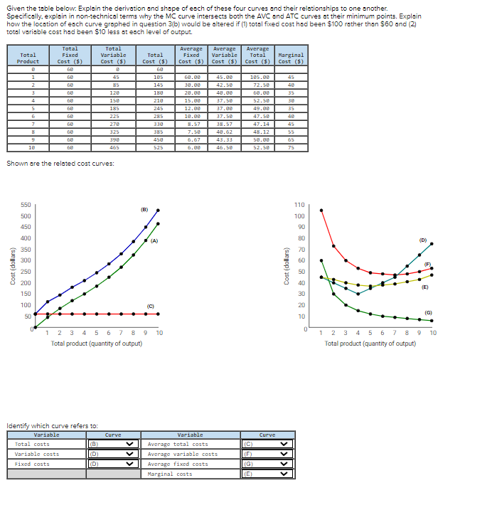
This image shows a table of cost data for various output levels and the corresponding cost curves plotted on two separate graphs. The top graph shows Total Cost (B), Variable Cost (A), and Fixed Cost (C). The bottom graph shows Average Total Cost (F), Average Variable Cost (G), Marginal Cost (E), and Average Fixed Cost (D).

This graph reveals the characteristic shapes of short-run cost curves. Let's formalize our understanding of why they look this way.

Cost Curves – Intermediate Microeconomics

This section from the Oregon State University textbook provides a clear graphical representation and explanation of the key short-run average and marginal cost curves.

Please read the subsection "Marginal, Average Fixed, Average Variable, and Average Total Cost Curves." Focus on the description of each curve's shape in Figure 8.3.

To summarize the key points on the shapes of the curves:

Average Fixed Cost (AFC) continuously declines. This is because the constant fixed cost is being "spread" over an increasing quantity of output ( $A F C = F C / Q$ ).
Marginal Cost (MC), Average Variable Cost (AVC), and Average Total Cost (ATC) are all typically U-shaped. This is a direct consequence of the law of diminishing marginal returns, which we discussed two lessons ago. Initially, as production starts, increasing marginal product of labor leads to falling marginal and average costs. Eventually, diminishing returns set in, causing marginal costs to rise, which in turn pulls the average costs up.
Average Total Cost (ATC) is the vertical sum of AFC and AVC. Notice in any such graph that the vertical distance between the ATC and AVC curves is the AFC. As output increases, this distance shrinks because AFC is falling.

The Critical Relationship: Marginal vs. Average Cost

Now, let's focus on the most important feature in these graphs: the intersection points. As you read in the previous section, the marginal cost curve always intersects both the AVC and ATC curves at their minimum points. This is not a coincidence but a mathematical necessity.

The reading provided a great analogy for this: your grade point average.

If your grade in the next course you take (the "marginal" grade) is below your current GPA (the "average"), it will pull your average down.
If your marginal grade is above your average, it will pull your average up.
Therefore, for your average to be at its lowest possible point, your marginal grade must be exactly equal to your average.

The same logic applies to costs. As long as the cost of the next unit (MC) is below the average cost (ATC), it pulls the average down. Once the MC rises above the ATC, it starts pulling the average up. The ATC curve can only be at its minimum at the exact point of transition, which is where $M C = A T C$ . The same holds true for the relationship between MC and AVC.

The Mathematical Proof

Given your background in statistics and probability, you'll appreciate that we can prove this relationship formally using calculus. To find the minimum of any function, we take its derivative and set it equal to zero. Let's do this for the Average Cost function, $A C (Q)$ .

The following video provides a concise and elegant proof of this principle.

Proof: Marginal Cost Equals Average Cost at Minimum of AC

This video, "Proof: Marginal Cost Equals Average Cost at Minimum of AC," walks through the calculus derivation step-by-step.

Please watch the entire video from the beginning to the end. The presenter applies the quotient rule for differentiation to the average cost function, AC = C(Q)/Q, and shows that setting the derivative to zero leads directly to the condition that marginal cost must equal average cost.

The steps of the proof are as follows:

Define Average Cost: $A C (Q) = \frac{C ( Q )}{Q}$
To find the quantity $Q$ that minimizes $A C$ , we must find where the derivative of $A C$ with respect to $Q$ is zero: $\frac{d ( A C )}{d Q} = 0$ .
Applying the quotient rule for derivatives, $\frac{d}{d x} (\frac{f ( x )}{g ( x )}) = \frac{f ^{'} ( x ) g ( x ) - f ( x ) g ^{'} ( x )}{[ g ( x ) ] ^{2}}$ , we get: $\frac{d ( A C )}{d Q} = \frac{\frac{d C ( Q )}{d Q} \cdot Q - C ( Q ) \cdot 1}{Q ^{2}} = 0$
For this fraction to be zero, the numerator must be zero: $\frac{d C ( Q )}{d Q} \cdot Q - C (Q) = 0$
Rearranging the terms gives: $\frac{d C ( Q )}{d Q} = \frac{C ( Q )}{Q}$
By definition, we know that $\frac{d C ( Q )}{d Q} = M C (Q)$ and $\frac{C ( Q )}{Q} = A C (Q)$ . Therefore, the condition for minimum average cost is: $M C (Q) = A C (Q)$

This confirms mathematically what the GPA analogy suggests intuitively. The exact same logic applies to finding the minimum of the Average Variable Cost curve.

Finding the Minimum Point in Practice

This relationship provides us with a powerful practical tool. If you are given a firm's cost function, you can find the output level that corresponds to the minimum average cost in two ways:

Derive the $A C$ function, take its derivative with respect to $Q$ , set it to zero, and solve for $Q$ .
Derive the $A C$ and $M C$ functions, set them equal to each other ( $A C = M C$ ), and solve for $Q$ .

Both methods will yield the same result. The second method is often algebraically simpler.

Let's watch a video that demonstrates how to find these minimum points for various cost curves using these calculus-based techniques.

Finding the Minimum Point on Cost Curves: ATC, AVC, and MC

The video "Finding the Minimum Point on Cost Curves" provides several worked examples using polynomial cost functions.

Watch the following segments to see this principle in action: First, watch the example of minimizing average variable cost from the beginning of the video. Here, the presenter finds the minimum by taking the derivative of the AVC function. Next, watch the example of minimizing average total cost from this segment. Finally, and most importantly, watch the segment from this part. It explicitly states that finding where AVC = MC is the same thing as finding where AVC is minimized, confirming our proof.

A Complete Example

Let's work through a full example that ties all these pieces together. Consider a firm with the following total cost function:

T C = 200 - 10 Q + 2 Q^{2}

Our goal is to find the quantity of output at which Average Total Cost (ATC) is at its minimum. We will use the $M C = A T C$ shortcut.

This image illustrates the step-by-step calculation for finding the minimum of the ATC curve by setting Marginal Cost equal to Average Total Cost for the function $TC = 200 - 10Q + 2Q^2$.

Following the logic in the image:

Find the Marginal Cost (MC): MC is the derivative of the Total Cost (TC) function. $M C = \frac{d T C}{d Q} = - 10 + 4 Q$
Find the Average Total Cost (ATC): ATC is the Total Cost function divided by Q. $A T C = \frac{T C}{Q} = \frac{200}{Q} - 10 + 2 Q$
Set MC equal to ATC: To find the minimum of the ATC curve, we set the two functions equal to each other. $- 10 + 4 Q = \frac{200}{Q} - 10 + 2 Q$
Solve for Q:
- First, we can add 10 to both sides, which cancels the constant term. $4 Q = \frac{200}{Q} + 2 Q$
- Next, subtract $2 Q$ from both sides. $2 Q = \frac{200}{Q}$
- Finally, multiply by $Q$ and solve. $2 Q^{2} = 200 ⟹ Q^{2} = 100 ⟹ Q = 10$

Thus, for this firm, average total cost is minimized when it produces 10 units of output. This is the efficient scale of production for the firm in the short run.

Conclusion

In this lesson, we moved beyond mere calculation to a deeper, analytical understanding of short-run costs. By plotting cost data, we visualized the characteristic shapes of the cost curves and uncovered the fundamental relationships between them.

Key Takeaways:

Short-run MC, AVC, and ATC curves are typically U-shaped due to the law of diminishing marginal returns.
The AFC curve is always downward sloping as fixed costs are spread over more units.
The MC curve intersects both the ATC and AVC curves at their respective minimum points.
This relationship is a mathematical necessity, which we proved using calculus by finding the minimum of the average cost function.
The condition $M C = A C$ (or $M C = A V C$ ) provides a direct method for calculating the output level that minimizes a firm's average costs.

In our next lesson, we will broaden our perspective to the long run, a timeframe in which all inputs are variable. We will introduce the long-run average cost (LRAC) curve and explore the important concepts of economies and diseconomies of scale.

Recommended resources