Long-Run Average Cost and Economies of Scale

From Short-Run Flexibility to Long-Run Planning

The key difference between the short run and the long run is the firm's ability to choose its scale of operation. In the short run, a firm is stuck with its current factory size (a fixed level of capital). In the long run, it can choose to build a small factory, a medium one, or a large one. Each of these choices corresponds to a different short-run average cost (SRAC) curve.

A rational, cost-minimizing firm will, for any given level of output it plans to produce, choose the factory size (i.e., the amount of capital) that allows it to produce that quantity at the lowest possible average cost. The long-run average cost curve is therefore constructed by tracing out the minimum possible average cost for every level of output.

The following video provides an excellent visualization of how the LRAC curve acts as a "lower envelope" to the family of possible SRAC curves.

As the video demonstrates, in the long run, the firm is unconstrained and can achieve an average cost that is less than or equal to the short-run average cost for any level of output.

Economies and Diseconomies of Scale

The U-shape of the typical LRAC curve is fundamental to understanding a firm's long-run production strategy. The shape reveals whether a firm experiences economies, diseconomies, or constant returns to scale.

Let's define these three regions based on the graph:

1. Economies of Scale: This occurs in the downward-sloping portion of the LRAC curve (the green region). As the firm increases its output, its long-run average cost per unit decreases. This is often due to:

   • Specialization: Larger operations allow for greater specialization of labor and machinery.
   • Indivisible Inputs: Some capital, like a large-scale packaging machine or a blast furnace, is not available in smaller sizes. Its high cost can only be justified at high output levels, where the cost is spread over many units.

2. Diseconomies of Scale: This occurs in the upward-sloping portion of the LRAC curve (the red region). Beyond a certain point, as a firm continues to expand, its long-run average cost per unit begins to increase. This is typically caused by:

   • Managerial Complexity: As a firm becomes very large, communication channels become longer, management becomes more bureaucratic, and coordinating all divisions becomes more difficult and costly.

3. Constant Returns to Scale: This is the flat portion of the LRAC curve between the other two regions (the yellow region). Here, long-run average cost remains constant as output changes.

The output level at which the LRAC curve reaches its minimum is known as the Minimum Efficient Scale (MES). This is the smallest scale at which a firm can operate to achieve the lowest possible average cost.

The Link Between Production and Costs

In a previous lesson, we touched upon returns to scale as a property of the production function. It describes how output changes when all inputs are scaled by a common factor. Economies of scale, conversely, is a property of the cost function. The two concepts are intrinsically linked.

• Increasing Returns to Scale (IRS): Doubling inputs more than doubles output. This means to double output, you need less than double the inputs (and thus less than double the cost). This causes average cost ($TC/Q$) to fall, leading to Economies of Scale.
• Decreasing Returns to Scale (DRS): Doubling inputs less than doubles output. To double output, you need more than double the inputs and cost. This causes average cost to rise, leading to Diseconomies of Scale.
• Constant Returns to Scale (CRS): Doubling inputs exactly doubles output. This means cost and output increase proportionally, so average cost remains constant, leading to Constant Returns to Scale.

For a Cobb-Douglas production function of the form $Q=A{K}^{\alpha }{L}^{\beta }$, you can quickly determine the returns to scale by examining the sum of the exponents, $\alpha +\beta$.

As the video explains:

• If $\alpha +\beta >1$, the function exhibits increasing returns to scale.
• If $\alpha +\beta =1$, it exhibits constant returns to scale.
• If $\alpha +\beta <1$, it exhibits decreasing returns to scale.

This gives you a powerful tool to predict the shape of the LRAC curve directly from the firm's production technology.

Calculating Long-Run Costs

Now, let's put this into practice by calculating a firm's long-run cost functions. Your background in optimization will be useful here, as the process involves finding the cost-minimizing combination of inputs for any given level of output.

The following resource provides a step-by-step mathematical example.

Let's summarize the procedure from the reading for finding the MES, as this directly addresses the learning outcome. Given a long-run total cost function, for example, $LRTC(Q)=160+10Q^2$:

1. Find Long-Run Average Cost (LRAC):

   $$LRAC=\frac{LRTC}{Q}=\frac{160}{Q}+10Q$$

2. Find Long-Run Marginal Cost (LRMC):

   $$LRMC=\frac{d(LRTC)}{dQ}=20Q$$

3. Find MES by setting LRAC = LRMC: The minimum of the LRAC curve occurs where it is intersected by the LRMC curve.

   $$\frac{160}{Q}+10Q=20Q$$ $$\frac{160}{Q}=10Q$$ $$160=10Q^2⟹Q^2=16⟹Q=4$$

Therefore, the Minimum Efficient Scale (MES) is 4 units.

• For output levels $Q<4$, the firm experiences economies of scale.
• For output levels $Q>4$, the firm experiences diseconomies of scale.

This calculation confirms how to identify the different regions of the LRAC curve.

Practice Question

Let's test your understanding with a graphical question.

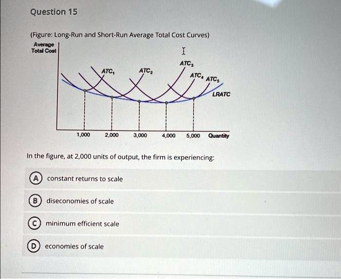
Looking at the graph, at an output level of 2,000 units, the firm is operating on the downward-sloping portion of its LRATC curve. What does this imply?

Conclusion

In this lesson, we transitioned from the constraints of the short run to the flexibility of the long run. We established that the long-run average cost (LRAC) curve represents the lowest possible cost of production for any given output level, acting as an envelope for all possible short-run cost curves.

Key Takeaways:

• The long run is a period where all inputs, including capital, are variable.
• The LRAC curve is the lower envelope of the infinite number of SRAC curves.
• The shape of the LRAC curve reveals economies of scale (downward-sloping), constant returns to scale (flat), and diseconomies of scale (upward-sloping).
• Minimum Efficient Scale (MES) is the output level that minimizes LRAC.
• These cost properties are directly linked to the production function's returns to scale (increasing, constant, or decreasing).
• Given a total cost function, we can calculate the MES by finding where $LRMC=LRAC$, which allows us to identify the regions of economies and diseconomies of scale.

In our next lesson, we will shift our focus from the cost side to the revenue side of the firm's operations. We will learn to calculate total, average, and marginal revenue, which are the final components needed before we can determine a firm's profit-maximizing level of output.