Calculating Deadweight Loss from Externalities

Part 1: Quantifying the Inefficiency of Negative Externalities

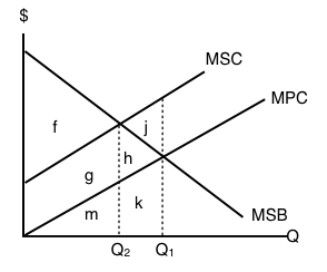
Let's begin with negative externalities, which are costs imposed on third parties. The classic example is pollution. When a firm produces a good, it considers its own private costs but often ignores the cost of the pollution it generates.

This leads to a divergence between private and social costs:

• Marginal Private Cost (MPC): The cost to the producer of making one more unit. This is represented by the firm's supply curve.
• Marginal External Cost (MEC): The cost imposed on others by the production of one more unit (e.g., health impacts of pollution).
• Marginal Social Cost (MSC): The true total cost to society of producing one more unit. It is the sum of the private and external costs: $MSC=MPC+MEC$.
• Marginal Social Benefit (MSB): The benefit to society from one more unit, which in the absence of a consumption externality, is simply the market demand curve.

In an unregulated market, equilibrium occurs where supply meets demand, meaning $MPC=MSB$. However, the socially efficient level of output is where the total social cost equals the social benefit: $MSC=MSB$.

Because $MSC>MPC$, the market equilibrium results in overproduction relative to the social optimum. This overproduction creates a deadweight loss (DWL), which represents the total loss of welfare to society. It is the cumulative amount by which the social cost exceeds the social benefit for each unit produced beyond the optimum.

To truly grasp this, we'll walk through a complete numerical calculation. The following video provides an excellent, step-by-step example.

As the video shows, the deadweight loss can be calculated as the area of a triangle:

Where:

• Base = The amount of overproduction ($Q_{\text{market}}-Q_{\text{optimal}}$).
• Height = The marginal external cost at the optimal quantity, which is also the divergence between the MSC and MSB curves at the market quantity ($MSC(Q_{\text{market}})-MSB(Q_{\text{market}})$).

This method provides a direct and efficient way to quantify the welfare loss, a critical first step in economic policy analysis. Let's try another example with a different set of equations to solidify the method.

Part 2: Quantifying the Inefficiency of Positive Externalities

Externalities can also be positive, meaning they confer benefits on third parties. Examples include education, research and development, and vaccinations. In these cases, the social benefit of an activity is greater than the private benefit to the individual.

The key terms are analogous to the negative externality case, but on the benefit side:

• Marginal Private Benefit (MPB): The benefit to the consumer of one more unit. This is the individual's demand curve.
• Marginal External Benefit (MEB): The benefit conferred on others by the consumption of one more unit.
• Marginal Social Benefit (MSB): The true total benefit to society from one more unit: $MSB=MPB+MEB$.
• Marginal Social Cost (MSC): The cost to society of producing one more unit, which we'll assume is just the market supply curve.

Here, the free market produces where $MPB=MSC$, but the social optimum is where $MSB=MSC$. Because $MSB>MPB$, the market equilibrium results in underproduction. Society misses out on net benefits because too few units are produced and consumed. This inefficiency is also a deadweight loss.

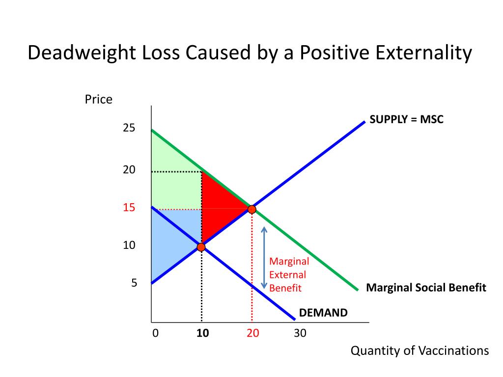
Let's use this graph to calculate the deadweight loss.

1. Identify Equilibria:

   • Market Equilibrium ($Q_{\text{market}}$): Where Demand (MPB) intersects Supply (MSC). This occurs at a quantity of 10 vaccinations and a price of $10.
   • Social Optimum ($Q_{\text{optimal}}$): Where Marginal Social Benefit (MSB) intersects Supply (MSC). This occurs at a quantity of 20 vaccinations and a price of $15.

2. Calculate Deadweight Loss:
   The DWL is the red triangle. Its area represents the net social benefit lost by not producing the units from 10 to 20.

   • Base = The amount of underproduction ($Q_{\text{optimal}}-Q_{\text{market}}$) = $20-10=10$.
   • Height = The divergence between the social benefit and social cost at the market quantity. At $Q=10$, the marginal social cost is $10 (from the supply curve), but the marginal social benefit is $20 (from the MSB curve). The height is therefore $MSB(10)-MSC(10)=20-10=10$.

   Now, we can calculate the area:

   $$DWL=\frac{1}{2}\times \text{Base}\times \text{Height}=\frac{1}{2}\times 10\times 10=\$50$$

   This $50 represents the total welfare lost because the market failed to account for the positive external benefits of vaccination, leading to under-consumption.

Part 3: A General Formula for Deadweight Loss

Whether the externality is positive or negative, on the production or consumption side, the principle for calculating deadweight loss is the same. The key is to identify the market quantity ($Q_{\text{market}}$) and the socially optimal quantity ($Q_{\text{optimal}}$).

The following resource provides a clear formula for calculating DWL in the case of a negative consumption externality (e.g., secondhand smoke), demonstrating the versatility of the concept.

The general formula for the area of the DWL triangle can be expressed as:

The absolute value signs ensure the formula works for both overproduction (negative externalities) and underproduction (positive externalities). This unified approach provides a robust tool for your analytical toolkit.

Conclusion

In this lesson, we have moved from simply identifying market failures to precisely measuring their impact. You now have the analytical framework to quantify the deadweight loss from both negative and positive externalities, a core skill for evaluating economic efficiency.

Key Takeaways:

• Externalities cause a divergence between private and social costs or benefits, leading to market failure.
• Negative externalities lead to overproduction, where $Q_{\text{market}}>Q_{\text{optimal}}$.
• Positive externalities lead to underproduction, where $Q_{\text{market}}<Q_{\text{optimal}}$.
• In both cases, the resulting inefficiency can be quantified as a deadweight loss (DWL).
• The DWL is calculated as the area of the triangle formed between the market quantity and the optimal quantity, bounded by the marginal social cost and marginal social benefit curves.

This foundational understanding of quantifying the problem is crucial for what comes next. In our next lesson, we will build directly on these calculations to determine the specific government interventions—namely Pigouvian taxes and subsidies—required to correct these externalities and restore market efficiency.