Correcting Externalities: Pigouvian Taxes & Subsidies

Correcting Negative Externalities: The Pigouvian Tax

When a negative externality exists, producers do not face the full cost of their actions. The Marginal Social Cost (MSC) of production is higher than the Marginal Private Cost (MPC). A Pigouvian tax aims to close this gap. It is a per-unit tax levied on the good or activity that generates the negative externality.

The key principle is that the tax should force the producer to "internalize the externality." To achieve the socially efficient outcome, the tax must be set equal to the marginal external cost (MEC) at the socially optimal level of output ($Q^{\ast }$).

Let's formalize this with a brief reading.

As the reading explains, the firm's new cost-minimizing choice will be where its new marginal cost, $MPC+\text{tax}$, equals the price. By setting the tax $t=MEC(Q^{\ast })$, we ensure that the firm chooses to produce exactly $Q^{\ast }$, where $MPC+MEC(Q^{\ast })=\text{price}$. Since $MPC+MEC=MSC$, this is equivalent to the condition for social optimality: $MSC=\text{price}$.

Visually, the tax shifts the MPC curve upward. The goal is to make this new, tax-inclusive private cost curve intersect the marginal benefit curve at the socially optimal quantity.

Calculating the Pigouvian Tax

Let's apply this to a numerical problem. We will use the same set of equations from a video in our previous lesson, but now focus on calculating the tax.

1. Find the Social Optimum ($Q^{\ast }$): First, we must find the socially optimal quantity by setting Marginal Social Cost (MSC) equal to Marginal Social Benefit (MSB).
2. Calculate the Tax: The tax is the value of the Marginal External Cost (MEC) at that optimal quantity, $Q^{\ast }$. Alternatively, it's the vertical distance between the MSC and MPC curves at $Q^{\ast }$.

The following video demonstrates this calculation.

Let's break down the calculation shown in the video.
The given equations are:

• Marginal Benefit (Demand): $P=24-Q$
• Marginal Private Cost: $MPC=2+Q$
• Marginal External Cost: $MEC=0.5Q$

From the video (and our previous lesson), the socially optimal quantity, where $MSB=MSC$, is $Q^{\ast }=8.8$.

To find the Pigouvian tax ($t$), we calculate the MEC at this quantity:
$t=MEC(Q^{\ast })=0.5\times Q^{\ast }$
$t=0.5\times 8.8=4.4$

Therefore, a tax of $4.40 per unit will cause the firm to reduce its production to the socially optimal level of 8.8 units. The presenter in the video uses an equivalent method by setting $P=MPC+t$ at the optimal quantity, which also yields $t=4.4$. This confirms the tax exactly equals the external cost at the efficient point.

Correcting Positive Externalities: The Pigouvian Subsidy

The logic for positive externalities is perfectly symmetrical. When an activity generates benefits for third parties (e.g., vaccination, R&D), its Marginal Social Benefit (MSB) is greater than the Marginal Private Benefit (MPB). The free market underproduces this good.

A Pigouvian subsidy is a per-unit payment to consumers or producers to encourage more of the activity. To be efficient, the subsidy must be set equal to the Marginal External Benefit (MEB) at the socially optimal quantity ($Q^{\ast }$).

This intervention raises the effective demand curve (MPB) or lowers the effective supply curve (MPC), causing the market to reach the efficient equilibrium at $Q^{\ast }$.

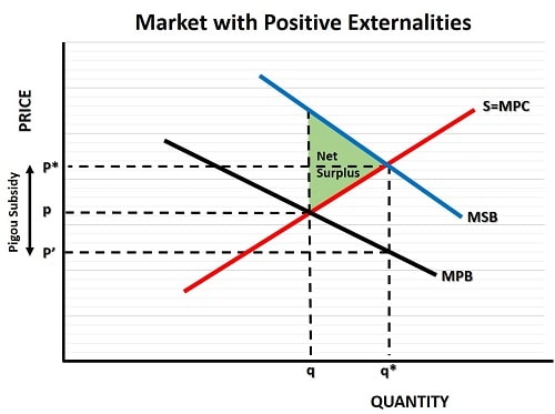
Calculating the Pigouvian Subsidy

The calculation process mirrors that of the tax:

1. Find the Social Optimum ($Q^{\ast }$): Find the quantity where Marginal Social Benefit (MSB) equals Marginal Social Cost (MSC).
2. Calculate the Subsidy: The subsidy is the value of the Marginal External Benefit (MEB) at that optimal quantity, $Q^{\ast }$. This is the vertical distance between the MSB and MPB curves at $Q^{\ast }$.

Let's watch a video that works through a full example.

Let's recap the video's calculation. The equations are:

• Marginal Private Benefit (MPB): $P=10-0.1Q$
• Marginal Cost (MC): $P=0.1Q$
• Marginal External Benefit (MEB): $MEB=5-0.05Q$

The socially optimal quantity is found by setting $MSB=MC$.
First, find MSB: $MSB=MPB+MEB=(10-0.1Q)+(5-0.05Q)=15-0.15Q$.
Setting $MSB=MC$:
$15-0.15Q=0.1Q$
$15=0.25Q$
$Q^{\ast }=60$

Now, we calculate the required subsidy ($s$) by finding the MEB at this optimal quantity:
$s=MEB(Q^{\ast })=5-0.05\times Q^{\ast }$
$s=5-0.05\times 60=5-3=2$

A subsidy of $2 per unit will incentivize consumers/producers to increase the quantity to the socially optimal level of 60 units. The video explains that this works because if consumers are given a $2 subsidy, their demand curve effectively becomes $P=(10-0.1Q)+2=12-0.1Q$. Setting this new demand equal to supply ($0.1Q$) gives $12=0.2Q$, or $Q=60$, confirming the subsidy achieves the desired outcome.

A More Formal View

Your quantitative background allows us to appreciate a more formal perspective on this principle. Corrective taxes and subsidies work because they force economic agents to confront the marginal social costs or benefits of their actions.

This resource highlights the robustness of the Pigouvian principle. Whether we are trying to reduce a negative activity like pollution or encourage a positive one, the solution is to set a price—a tax or a subsidy—on the externality itself, equal to its marginal effect at the optimal level of activity.

Conclusion

You have now learned not only how to measure the problem of externalities but also how to solve it with precision. By correctly calculating and applying Pigouvian taxes and subsidies, a government can align private incentives with social welfare, correct the market failure, and eliminate the deadweight loss.

Key Takeaways:

• A Pigouvian tax is used to correct a negative externality. Its optimal value is equal to the Marginal External Cost at the socially optimal quantity ($t=MEC(Q^{\ast })$).
• A Pigouvian subsidy is used to correct a positive externality. Its optimal value is equal to the Marginal External Benefit at the socially optimal quantity ($s=MEB(Q^{\ast })$).
• These interventions "internalize the externality" by adjusting the marginal costs or benefits faced by private decision-makers, guiding them toward the socially efficient level of output.
• The calculation requires first finding the social optimum ($Q^{\ast }$) and then evaluating the marginal externality at that specific quantity.

In our next lesson, we will explore another major category of market failure: public goods. We will see why markets often fail to provide them and introduce a new quantitative tool, the Samuelson condition, to determine the efficient level of provision.