Introduction
In our last lesson, we established that in market economies, the price mechanism is the central nervous system that coordinates resource allocation. This raises a critical question: what determines the price of a good or service in the first place? To answer this, we will now build the most fundamental tool in all of economics: the model of supply and demand.
This lesson will guide you through the construction of demand and supply curves, translating them from simple tables of data into graphical representations and, crucially for your analytical interests, into linear equations. You will learn to distinguish between a movement along a curve, caused by a change in price, and a shift of the entire curve, caused by other factors. This foundational understanding is essential, as it underpins the analysis of nearly every market you will encounter in this course.
The Demand Side of the Market
Demand is not just about wanting something; in economics, it represents the quantity of a good that consumers are both willing and able to purchase at various prices over a specific period, holding all other factors constant (an assumption economists call ceteris paribus).
The relationship between price and quantity demanded can be represented in three ways:
- A demand schedule: A table showing quantity demanded at different prices.
- A demand curve: A graph of the demand schedule.
- A demand equation: A mathematical function that describes the curve.
Let's begin with a foundational reading that explains how to move from the concept of demand to a plotted curve.
[PDF] DEMAND AND SUPPLY CURVES - Linear Equations & Graphs ...
This document provides a clear, step-by-step guide to understanding and plotting demand curves. It also highlights an important convention in economics that can be a source of confusion.
Please read the section titled "Demand Curves". As you read, pay close attention to two key points: The Law of Demand: the inverse relationship between price and quantity demanded. The axis convention: Economists plot price (the independent variable, x) on the vertical axis and quantity (the dependent variable, y) on the horizontal axis. This is a reversal of the standard mathematical convention.
As the reading explains, the demand curve is typically downward-sloping, reflecting the Law of Demand. When this relationship is linear, we can express it with a simple equation.
From a Schedule to an Equation
The standard form of a linear demand equation is:
Where:
- is the quantity demanded.
- is the price.
ais the horizontal intercept, representing the quantity demanded if the price were zero.-bis the slope of the demand function (). Note that because of the axis-flipping convention, the slope of the plotted curve is the reciprocal, .
Your background in statistics makes you well-equipped to derive these parameters from data. Consider the following demand schedule for coffee:
| Price (P) | Quantity Demanded (Qd) |
|---|---|
| $3 | 34 |
| $6 | 28 |
To find the slope, b, we calculate the change in quantity over the change in price:
So, . Our equation is now .
To find the intercept, a, we substitute any of the price-quantity pairs into the equation. Using the first pair (P=3, Qd=34):
Thus, the demand equation is . This process is analogous to finding the equation of a line from two data points.
The following video provides an excellent visual walkthrough of how to plot a demand curve from its equation by finding the axis intercepts.
How to Draw the DEMAND CURVE (Using the DEMAND EQUATION) | Think Econ
This video from Think Econ demonstrates a practical approach to graphing a linear demand equation.
Watch the segment from the beginning until the end of the example. The instructor shows how to find the quantity intercept (by setting P=0) and the price intercept (by setting Q=0) to anchor the curve. They also show how to find other points on the curve.
Shifts in the Demand Curve
The ceteris paribus assumption we made earlier is crucial. It allows us to isolate the relationship between price and quantity. But what happens when those "other things" change?
A change in any factor other than the good's own price that affects consumers' willingness or ability to buy will cause the entire demand curve to shift. This is called a change in demand. A movement along the curve is a change in quantity demanded caused only by a price change.
The main non-price determinants that shift the demand curve are:
- Consumer Income: For a normal good, higher income increases demand (shifts right). For an inferior good, higher income decreases demand (shifts left).
- Prices of Related Goods:
- Substitutes: If the price of a substitute (e.g., tea) increases, the demand for the original good (e.g., coffee) increases (shifts right).
- Complements: If the price of a complement (e.g., sugar) increases, the demand for the original good (e.g., coffee) decreases (shifts left).
- Tastes and Preferences: A change in fashion or a health report can increase or decrease demand.
- Expectations: If you expect the price to rise next week, you might buy more today, increasing current demand.
- Number of Buyers: More consumers in the market increases demand.
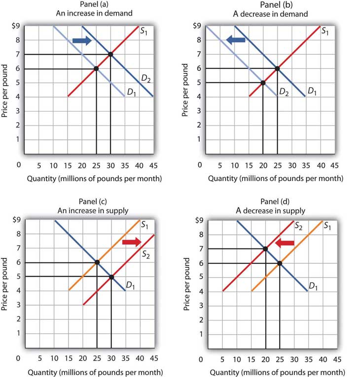
The image below illustrates the concept of shifts. A rightward shift (from D₁ to D₂) signifies an increase in demand, meaning more is demanded at every price. A leftward shift (from D₂ to D₁) signifies a decrease.
The Supply Side of the Market
Now let's turn to the producers. Supply represents the quantity of a good that producers are willing and able to offer for sale at various prices over a given period, ceteris paribus.
Like demand, supply can be represented by a schedule, a curve, and an equation. The key difference is the Law of Supply: there is a positive relationship between price and quantity supplied. As the price of a good rises, producers have a greater incentive to produce and sell more of it. This gives the supply curve its characteristic upward slope.
The linear supply equation is:
Where:
- is the quantity supplied.
cis the horizontal intercept (which may be negative, implying that the price must be above a certain level for any quantity to be supplied).dis the slope (), which is positive.
Shifts in the Supply Curve
Just as with demand, we must distinguish between a movement along the supply curve (caused by a change in the good's own price) and a shift of the entire curve (a change in supply).
The main non-price determinants that shift the supply curve are:
- Input Prices: A decrease in the cost of raw materials, labor, or machinery lowers production costs and increases supply (shifts right).
- Technology: Improvements in technology that make production more efficient increase supply (shifts right).
- Number of Sellers: More producers entering the market increases supply (shifts right).
- Expectations: If producers expect prices to be much higher in the future, they might reduce the quantity they offer for sale today, decreasing current supply (shifts left).
In the image "Changes in Demand and Supply" above, Panel (c) shows an increase in supply (rightward shift), while Panel (d) shows a decrease in supply (leftward shift). Notice that for supply, a leftward shift appears to move the curve "up." Always remember the mnemonic: "less is left." A shift to the left means less quantity is supplied at any given price.
Market Equilibrium: Where Supply Meets Demand
Having constructed the two sides of the market, we can now bring them together. The point where the supply and demand curves intersect is the market equilibrium. The price at this intersection is the equilibrium price, and the quantity is the equilibrium quantity.
At equilibrium, the quantity that buyers are willing and able to buy is exactly equal to the quantity that sellers are willing and able to sell (). There is no pressure for the price to change.
To see how to plot both curves and identify this equilibrium point, let's watch a final video. This will serve as a bridge to our next lesson, where we will solve for equilibrium algebraically.
This video from Constantin Bürgi provides a complete example of drawing both supply and demand curves from their equations and finding the market equilibrium.
Please watch this video in its entirety. It will recap several concepts from this lesson and give you a preview of the next. Focus on: Rearranging the standard Q=f(P) equations into the P=f(Q) format for plotting, as discussed in the first reading. This process is known as finding the inverse demand and supply functions. How the two curves are drawn on the same axes. Watch this section closely. The conceptual setup for finding equilibrium: setting quantity demanded equal to quantity supplied. This calculation is exactly what we will be doing in detail in the next lesson.
Conclusion
In this lesson, you have learned to construct the fundamental building blocks of market analysis. We moved from schedules of data to graphical curves and then to algebraic equations for both supply and demand. You are now able to translate between these three representations and, critically, to distinguish between movements along the curves and shifts of the curves themselves.
Key Takeaways:
- Demand curves represent the relationship between price and the quantity consumers are willing and able to buy. They are downward-sloping and can be expressed as .
- Supply curves represent the relationship between price and the quantity producers are willing and able to sell. They are upward-sloping and can be expressed as .
- A change in a good's own price causes a movement along its supply or demand curve.
- A change in a non-price determinant (like income, technology, or input costs) causes a shift of the entire curve.
- The intersection of the supply and demand curves determines the market equilibrium price and quantity.
We ended with a preview of how to find this equilibrium point. In our next lesson, we will formalize this process. You will apply the equations you've learned to derive today to algebraically calculate market equilibrium and analyze how that equilibrium changes when the supply or demand curves shift.