Equilibrium: Supply, Demand, and Shifts

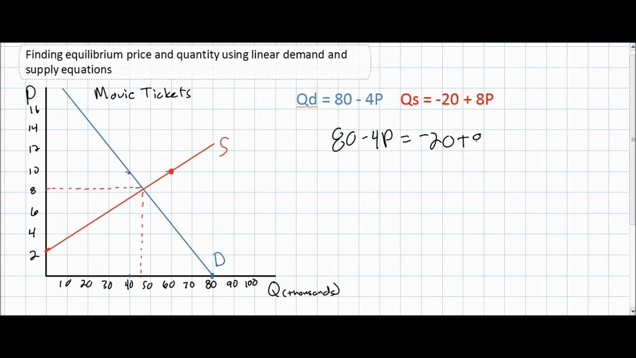
Finding Equilibrium Algebraically

The market is in equilibrium when the quantity consumers wish to buy is exactly equal to the quantity producers wish to sell. This simple but powerful condition, $Q_d=Q_s$, is the key to solving the system. Since both the demand and supply equations are expressed in terms of price ($P$), setting them equal to each other creates a single equation with a single unknown variable: the equilibrium price.

The process involves three straightforward steps:

1. Set $Q_d=Q_s$. This establishes the equilibrium condition.
2. Solve for $P$. This gives you the equilibrium price, often denoted as $P^{\ast }$.
3. Substitute $P^{\ast }$ back into either the demand or supply equation to find the equilibrium quantity, $Q^{\ast }$. Solving with both equations is a useful way to check your work; the result should be the same.

The following video provides a clear, step-by-step demonstration of this algebraic method, without relying on graphs.

To solidify your understanding and see more worked examples, the following reading provides a concise review of the necessary algebra and applies it to several supply and demand problems.

Analyzing Shifts in Equilibrium (Comparative Statics)

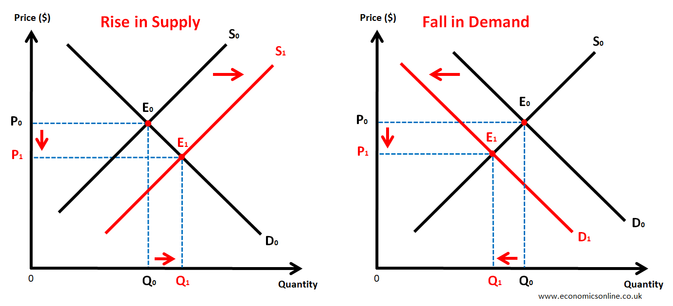
The real power of this algebraic approach becomes apparent when we analyze changes in the market. In the last lesson, we discussed how non-price determinants (like consumer income or input costs) cause the entire demand or supply curve to shift. Algebraically, these shifts are represented by changes in the parameters of the demand ($Q_d=a-bP$) or supply ($Q_s=c+dP$) equations—most often the intercept terms, a or c.

When a curve shifts, a new equilibrium price and quantity will emerge. By modifying the relevant equation and re-solving the system, we can precisely calculate the impact of the shift.

Let's work through an example. Suppose a market is described by:

• Demand: $Q_d=200-10P$
• Supply: $Q_s=-40+20P$

Setting $Q_d=Q_s$:
$200-10P=-40+20P$
$240=30P$
$P^{\ast }=8$
And substituting back: $Q^{\ast }=200-10(8)=120$.

Now, imagine an improvement in technology increases supply by 60 units at every price. The supply curve shifts right. The new supply equation becomes:

• New Supply: $Q_s^{\prime }=(-40+20P)+60=20+20P$

To find the new equilibrium, we set the original demand equal to the new supply:
$200-10P=20+20P$
$180=30P$
$P^{\prime }=6$
And the new quantity is $Q^{\prime }=20+20(6)=140$.

The technological improvement caused the equilibrium price to fall from $8 to $6, and the equilibrium quantity to rise from 120 to 140 units, just as the graphical analysis would predict.

For further practice, Exercise 2 in the following document shows how an increase in demand (from new export markets) affects the equilibrium in the wheat market.

A More General Approach: Comparative Statics

Your background in statistics and mathematical modeling will appreciate a more general way to think about these shifts. Instead of modeling a shift with a specific number, we can include the underlying factor as a parameter in our equations. This is the essence of comparative statics.

For example, the supply of a product might depend not only on its own price ($P$) but also on the price of an input, like capital ($R$). A supply function could be written as $Q_s=f(P,R)$. We can then solve for the equilibrium price and quantity as functions of $R$, i.e., $P^{\ast }(R)$ and $Q^{\ast }(R)$.

Using calculus, we can then find the derivative of the equilibrium price with respect to the input price, $\frac{d{P}^{\ast }}{dR}$. This tells us precisely how much the equilibrium price changes for a one-unit change in the price of capital. This approach provides a powerful and general way to analyze the sensitivity of a market equilibrium to external factors.

The following video demonstrates this advanced technique.

Conclusion

In this lesson, you have mastered the fundamental quantitative skill of solving for market equilibrium. By moving beyond graphical analysis to algebraic solutions, you can now calculate precise equilibrium outcomes and, crucially, determine the exact impact of market shocks.

Key Takeaways:

• The market equilibrium condition is $Q_d=Q_s$.
• By setting the linear demand and supply equations equal, you can solve for the equilibrium price ($P^{\ast }$) and subsequently the equilibrium quantity ($Q^{\ast }$).
• Shifts in demand or supply, caused by changes in non-price determinants, are modeled as changes to the parameters of the equations (typically the intercepts).
• Calculating the new equilibrium after a parameter change is a method known as comparative statics, which allows for precise analysis of market shocks.
• For a more general analysis, equilibrium outcomes can be expressed as functions of exogenous variables, and calculus can be used to determine their rate of change.

You are now equipped with the core analytical toolset for supply and demand analysis. In our next lesson, we will build directly on this by using the equilibrium price and quantity to measure the benefits that consumers and producers gain from market transactions, a concept known as consumer and producer surplus.