Calculating Consumer and Producer Surplus

Introduction

In our last lesson, you mastered the algebraic method for finding the market equilibrium price and quantity, $(P^{*}, Q^{*})$ . This equilibrium represents the point where the plans of buyers and sellers perfectly align. Now, we will build directly upon that foundation to answer a crucial question: how much value do consumers and producers actually get from participating in this market?

This lesson introduces the concepts of consumer surplus and producer surplus, which are the standard economic tools for measuring the welfare or gains from trade for each side of the market. Given your background in quantitative analysis, you'll appreciate that we will move beyond simple geometric shapes to a more robust and universally applicable method using definite integrals. This will allow us to calculate these surpluses precisely for any given supply and demand functions, a skill essential for the CB2 exam and for understanding the efficiency of market outcomes.

The Concepts of Consumer and Producer Surplus

At its heart, the concept of surplus is about the difference between what someone is willing to do and what they actually have to do.

Consumer Surplus (CS) is the total benefit or value that consumers receive beyond what they pay for a good. The demand curve reveals the maximum price consumers are willing to pay for each unit. Since everyone in the market buys at the same equilibrium price, many consumers end up paying less than their maximum willingness to pay. The sum of these individual gains is the consumer surplus.
Producer Surplus (PS) is the total benefit or revenue that producers receive beyond their cost of production. The supply curve reveals the minimum price producers are willing to accept for each unit. Since all producers in the market sell at the same equilibrium price, many receive more than their minimum acceptable price. This difference, summed across all units sold, is the producer surplus.

Graphically, these concepts are represented by the areas between the demand/supply curves and the equilibrium price line, up to the equilibrium quantity.

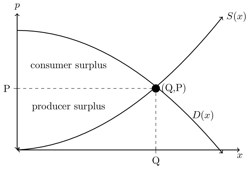
This graph illustrates the consumer surplus as the area below the demand curve D(x) and above the equilibrium price P. The producer surplus is the area above the supply curve S(x) and below the equilibrium price P, both calculated up to the equilibrium quantity Q.

For simple linear supply and demand curves, these areas are triangles, and their area can be calculated using the familiar formula $\frac{1}{2} \times base \times height$ . While useful for intuition, this method is limited. A more powerful approach uses calculus.

From Riemann Sums to Integral Formulas

The idea of summing up the "surplus" on each individual unit until the equilibrium quantity is reached should resonate with the concept of integration. The total willingness to pay can be thought of as the sum of the prices for infinitesimally small increments of quantity, which is precisely the definition of a definite integral.

The following document provides a rigorous derivation of the integral formulas for consumer and producer surplus, starting from the concept of a Riemann sum. Given your background in probability and statistics, you should find this formal development particularly insightful.

application of the integral i: consumer and producer surplus

This reading from the University of British Columbia derives the formulas for consumer and producer surplus from first principles. It elegantly connects the economic intuition to the mathematical formalism of calculus.

Please read the section titled Surplus and Integrals. Pay close attention to how the author approximates the total amount consumers would be willing to pay using a sum (a Riemann sum) and then takes the limit to arrive at a definite integral. This will solidify your understanding of why integration is the correct tool here.

As the reading demonstrates, the formal definitions for consumer and producer surplus are:

Consumer Surplus (CS):

C S = \int_{0}^{q_{e}} D (q) d q - p_{e} q_{e}

This formula states that consumer surplus is the total area under the demand curve from 0 to the equilibrium quantity $q_{e}$ (the total utility in monetary terms), minus the actual amount spent, which is the rectangle $p_{e} q_{e}$ .

Producer Surplus (PS):

P S = p_{e} q_{e} - \int_{0}^{q_{e}} S (q) d q

Similarly, producer surplus is the total revenue $p_{e} q_{e}$ minus the area under the supply curve (the total marginal cost of production).

The sum of these two, Social Surplus ( $S S = C S + P S$ ), represents the total gains from trade in the market.

A Step-by-Step Calculation

Let's now walk through a complete example that ties everything together: finding equilibrium, and then applying the integral formulas to calculate the surpluses.

The following video provides an excellent demonstration. It starts with demand and supply functions, calculates the equilibrium point (as we did in the last lesson), and then systematically computes the consumer, producer, and social surplus using the integral formulas.

Solving for Consumer, Producer, and Social Surplus using Integration

This video, "Solving for Consumer, Producer, and Social Surplus using Integration" by Justin Eloriaga, is a comprehensive walkthrough of the entire process.

Please watch from the beginning of the example. The video covers four key steps that you should focus on: Finding Equilibrium: First, he solves for p_e and q_e by setting the demand and supply equations equal to each other. Calculating Consumer Surplus: He sets up and solves the definite integral for CS using the formula we just discussed. Calculating Producer Surplus: He does the same for PS. Calculating Social Surplus: Finally, he sums the two to find the total welfare.

Practice with a Non-Linear Example

The true advantage of the integral method is its applicability to any form of demand or supply curve, not just linear ones. Let's apply this to a case with a non-linear demand function.

The document you read earlier also contains a worked example. This problem requires solving a quadratic equation to find equilibrium and evaluating an integral involving a natural logarithm—a great way to practice your calculus.

application of the integral i: consumer and producer surplus

This is the example problem from the same PDF we used for the derivation.

Please read the section titled Example. Follow the steps for finding the equilibrium quantity and price first. Then, study how the CS and PS integrals are set up and solved. Notice that the CS calculation results in a ln(q+1) term, showcasing a common integration result.

For even more practice with different functional forms (such as quadratic supply functions), you can review the exercises in the document "MATH 134 Calculus 2 with FUNdamentals - Applications to Economics" (resource LINK).

Conclusion

In this lesson, you have learned how to quantify the benefits that consumers and producers receive from market transactions. By building on your knowledge of equilibrium and leveraging your analytical skills, you can now calculate consumer and producer surplus for any given supply and demand functions.

Key Takeaways:

Consumer Surplus (CS) measures the net benefit to buyers, defined as the difference between their maximum willingness to pay and the actual market price.
Producer Surplus (PS) measures the net benefit to sellers, defined as the difference between the market price and their minimum willingness to accept.
While these can be visualized as triangles in simple linear cases, the robust method for calculation uses definite integrals.
The integral formulas are:
- $C S = \int_{0}^{q_{e}} D (q) d q - p_{e} q_{e}$
- $P S = p_{e} q_{e} - \int_{0}^{q_{e}} S (q) d q$

These surplus measures are not just abstract calculations; they form the bedrock of welfare economics. In our next lesson, we will use them as a benchmark to analyze how government interventions, such as price ceilings and price floors, affect market outcomes and lead to a loss of total surplus, a concept known as deadweight loss.

Recommended resources