Price Controls: Ceilings, Floors, and Their Market Impacts

Introduction

In our previous lesson, you learned to calculate consumer and producer surplus, which together measure the total welfare, or gains from trade, created in a free market. This equilibrium outcome is considered efficient because it maximizes this total surplus. Now, we will explore what happens when a government intervenes and prevents the market from reaching that equilibrium price.

This lesson addresses how government-imposed price ceilings (maximum prices) and price floors (minimum prices) disrupt market outcomes. You will learn to calculate the resulting shortages or surpluses, the redistribution of welfare between consumers and producers, and the creation of deadweight loss—a measure of the economic efficiency lost due to the intervention. Your analytical skills will be essential as we quantify these effects step-by-step using supply and demand equations.

The Impact of Price Ceilings

A price ceiling is a legal maximum on the price at which a good can be sold. For a price ceiling to have any effect, it must be binding, meaning it is set below the free-market equilibrium price ( $p_{e}$ ). If it were set above $p_{e}$ , the market would naturally settle at $p_{e}$ anyway, and the ceiling would be irrelevant.

When a binding price ceiling is imposed, two main things happen:

The lower price increases the quantity demanded but decreases the quantity supplied. This creates a shortage, where $Q_{D} > Q_{S}$ .
Since sellers are only willing to supply the smaller quantity at the ceiling price, this lower quantity becomes the amount actually bought and sold in the market. We say the "short side" of the market (in this case, supply) determines the quantity transacted.

This intervention reallocates surplus and creates inefficiency. Some consumers who can still buy the good are better off because they pay a lower price. However, producers are worse off. Critically, some mutually beneficial trades that would have occurred at quantities between the new, lower quantity and the original equilibrium quantity no longer happen. The value of these lost trades is the deadweight loss (DWL).

This graph shows a binding price ceiling set at P2, below the equilibrium price Pe. At P2, quantity supplied is Q1 while quantity demanded is Q3, creating a shortage. The quantity traded falls to Q1. The blue area is the new producer surplus, the orange area is the new consumer surplus, and the grey triangle represents the deadweight loss.

Calculating the Effects of a Price Ceiling

The best way to understand the full impact is to work through a numerical example. The following video solves a problem by first finding the market equilibrium and initial surpluses, and then recalculating everything after a price ceiling is imposed. This process is exactly what you'll need for your CB2 exam.

Consumer Surplus, Producer Surplus,& Deadweight Loss before and after imposing the price ceiling?

This video from ECON MATHS provides a complete, step-by-step calculation of consumer surplus, producer surplus, and deadweight loss before and after a price ceiling.

Please watch the entire video. The process can be broken down into these key stages: Before Intervention (Equilibrium & Surplus): The instructor first calculates the equilibrium price and quantity, then finds the price-axis intercepts for the supply and demand curves. He uses these values to calculate the initial consumer and producer surplus as the areas of two triangles. This should be a good review from our last lesson. After Intervention (New Surpluses): A price ceiling is imposed. He finds the new quantity transacted by plugging the ceiling price into the supply function. This is the "short side" of the market. He calculates the new, smaller producer surplus. To calculate the new consumer surplus (the trapezoid shape), he first finds the price on the demand curve corresponding to the new limited quantity. This allows him to break the trapezoid into a rectangle and a triangle and sum their areas. Deadweight Loss (DWL Calculation): Finally, he identifies the deadweight loss triangle and calculates its area. Notice that the sum of the new CS, new PS, and the DWL equals the original total surplus.

The Impact of Price Floors

A price floor is a legal minimum on the price at which a good can be sold. A binding price floor is set above the equilibrium price. The most common example is a minimum wage in the labor market.

When a binding price floor is imposed:

The higher price decreases the quantity demanded but increases the quantity supplied, creating a surplus, where $Q_{S} > Q_{D}$ .
The quantity actually transacted is determined by the "short side" of the market, which is now the quantity demanded at the floor price.

This leads to a different redistribution of surplus. Producers who can still sell the good are better off due to the higher price. Consumers are unambiguously worse off. Again, the value of trades that no longer occur constitutes the deadweight loss.

This graph illustrates a binding price floor set at Pf, above the equilibrium price Pe. This creates a surplus, as quantity supplied (Qs) exceeds quantity demanded (Qd). The quantity traded falls to Qd. The purple area is the new consumer surplus, the orange area is the new producer surplus, and the red triangle is the deadweight loss.

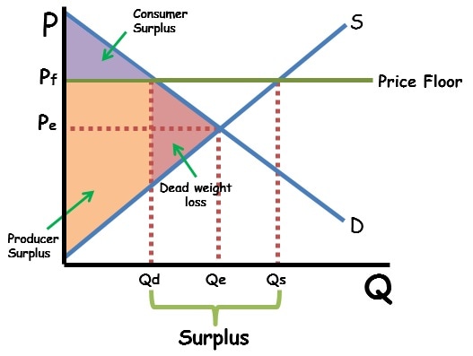
Calculating the Effects of a Price Floor

The calculation process for a price floor is symmetric to that of a price ceiling. You must first identify the new quantity transacted and then use that to find the new surplus areas and the deadweight loss.

The following video provides a concise guide to this calculation.

How to Calculate Deadweight Loss (with a Price Floor) | Think Econ

This video from the channel Think Econ, "How to Calculate Deadweight Loss (with a Price Floor)", focuses specifically on the quantitative impact of a price floor.

Watch the video from the start of the calculation. Pay close attention to these critical steps: Find Equilibrium (Step 1): He starts by finding the equilibrium price and quantity, P^* and Q^*. Find New Quantity (Step 2): With the price floor imposed, he finds the new, lower quantity traded by plugging the floor price into the demand function (the "short side"). Find Key Prices for DWL (Step 3): To find the height of the DWL triangle, he needs the price on the supply curve that corresponds to the new quantity. He finds this by plugging the new quantity into the supply function. Calculate DWL (Step 4): With the base (change in quantity) and height (change in price) of the DWL triangle identified, he calculates its area.

A Worked Example: Price Floor in the Milk Market

To solidify your understanding, let's review a detailed written example. The following document works through a problem involving a price floor for milk. This will reinforce the steps you saw in the video.

[PDF] quiz 1 practice problem solutions

This document from Syracuse University provides worked solutions to several economics problems. We will focus on the price floor example.

Read through the solution for Question 2 (a-c), which you can find by searching for the text Milk Market Example. Follow the author's steps: Part (a): Calculation of the initial equilibrium. Part (b): Calculation of the new quantity sold after the price floor is imposed. Note that this is found from the demand equation. Part (c): Calculation of the changes in consumer surplus, producer surplus, and the deadweight loss. Pay special attention to how the new producer surplus (the trapezoid B + C + D) is calculated by first finding the price on the supply curve at the new quantity of 19. This is a crucial step that is often overlooked.

Conclusion

In this lesson, you've moved from analyzing an efficient, free-market equilibrium to quantifying the inefficiencies caused by government price controls. You are now equipped to analyze the full spectrum of effects from these policies.

Key Takeaways:

A binding price ceiling (below equilibrium) causes a shortage ( $Q_{D} > Q_{S}$ ). The quantity transacted is determined by suppliers.
A binding price floor (above equilibrium) causes a surplus ( $Q_{S} > Q_{D}$ ). The quantity transacted is determined by demanders.
In both cases, the quantity of the good traded in the market decreases.
Deadweight Loss (DWL) arises in both scenarios. It represents the total surplus lost from transactions that are no longer made, signifying a loss of economic efficiency.
The calculation procedure is:
1. Find the original market equilibrium ( $p_{e}, q_{e}$ ).
2. Identify the new quantity transacted ( $q ˉ$ ) by plugging the controlled price into the "short side" of the market's equation (supply for a ceiling, demand for a floor).
3. Calculate the new CS and PS based on the controlled price and new quantity. This may require finding the price on the "long side" curve at $q ˉ$ .
4. Calculate the DWL as the area of the triangle formed by the reduction in quantity and the gap between the demand and supply curves over that range.

In our next module, we will begin our study of elasticity. This concept measures the responsiveness of quantity demanded or supplied to changes in price and other factors. Understanding elasticity will add a new layer of depth to our analysis, as it helps determine the magnitude of the shortages, surpluses, and deadweight losses that result from the price controls we've studied today.

Recommended resources