Price Elasticity of Demand: Point and Midpoint Methods

Introduction

In our last lesson, we analyzed how price controls like ceilings and floors disrupt market equilibrium, leading to shortages, surpluses, and deadweight loss. We saw that a change in price causes a change in the quantities producers are willing to supply and consumers are willing to buy. This naturally leads to a crucial question: by exactly how much does quantity demanded respond to a price change?

This lesson introduces the concept of price elasticity of demand, a fundamental tool in economics for quantifying this responsiveness. Your strong background in statistics and quantitative reasoning will be particularly useful here, as we will define elasticity using precise mathematical formulas. We will cover the two primary methods for its calculation that are essential for your CB2 exam: the point elasticity method, which uses calculus for precision at a single point on the demand curve, and the midpoint method, used to measure average elasticity over a price range.

Defining Price Elasticity of Demand

At its core, price elasticity of demand ( $E_{d}$ ) measures the sensitivity of quantity demanded to a change in price. It is formally defined as the percentage change in quantity demanded divided by the percentage change in price.

E_{d} = \frac{% Change in Quantity Demanded}{% Change in Price} = \frac{%Δ Q _{d}}{%Δ P}

Using percentages makes elasticity a unitless measure, allowing for comparisons across different goods and markets, regardless of the units used for price (e.g., dollars, euros) or quantity (e.g., kilograms, gallons).

To begin, let's watch a short segment that introduces this core concept and provides a helpful analogy.

Price elasticity of demand using the midpoint method | Elasticity | Microeconomics | Khan Academy

This video from Khan Academy, titled "Price elasticity of demand using the midpoint method", clearly explains the "what" and "why" of elasticity.

Please watch the first four minutes of the video, covering the definition and the helpful "rubber band" analogy for elastic vs. inelastic demand (What is Elasticity?). Focus on why economists use percentage changes rather than absolute changes.

As the video explains, if a small percentage change in price leads to a large percentage change in quantity demanded, we say demand is elastic. If it leads to a small percentage change, demand is inelastic. Now, let's turn to the formal methods of calculation.

Method 1: Point Elasticity

The point elasticity method calculates elasticity at a specific point on the demand curve. This requires that we know the mathematical form of the demand function, $Q = f (P)$ . This method will likely feel intuitive given your background, as it employs calculus for a precise, instantaneous measure of responsiveness.

Let's expand the definition of elasticity:

E_{d} = \frac{Δ Q / Q}{Δ P / P}

Rearranging this gives:

E_{d} = \frac{Δ Q}{Δ P} \cdot \frac{P}{Q}

For an infinitesimally small change in price, the ratio $\frac{Δ Q}{Δ P}$ becomes the derivative of the demand function with respect to price, $\frac{d Q}{d P}$ . This gives us the point elasticity formula:

E_{d} = \frac{d Q}{d P} \cdot \frac{P}{Q}

Since the law of demand implies that $\frac{d Q}{d P}$ is negative, $E_{d}$ will also be negative. For interpretation, economists often take the absolute value, $∣ E_{d} ∣$ .

The following video provides an excellent walkthrough of deriving this formula and applying it to a linear demand curve.

price elasticity of demand (calculus)

The video "price elasticity of demand (calculus)" from Economics in Many Lessons shows how to move from the basic definition to the calculus-based formula and apply it.

Watch the first seven minutes, which cover two key parts: Derivation (Formula Derivation): Pay close attention to how the \Delta notation is replaced with derivative notation to arrive at the point elasticity formula. Example Calculation (First Example): Follow the step-by-step calculation for finding the elasticity at a price of $4. Notice the two steps: first find the derivative, then evaluate the full expression at the specific price and corresponding quantity.

As the video demonstrates, calculating point elasticity is a clear process:

If necessary, solve the demand equation for $Q$ to get it in the form $Q = f (P)$ .
Find the derivative, $\frac{d Q}{d P}$ . This is the slope of the demand function when plotted with Q on the y-axis and P on the x-axis. Note that most demand curves in economics are plotted with P on the y-axis (inverse demand), so $\frac{d Q}{d P}$ is the reciprocal of the slope of the graphed line.
Substitute the specific price $P$ into the demand equation to find the corresponding quantity $Q$ .
Plug $\frac{d Q}{d P}$ , $P$ , and $Q$ into the elasticity formula.

For a general linear demand curve $Q = a - b P$ , the derivative $\frac{d Q}{d P}$ is simply $- b$ . Thus, the formula becomes $E_{d} = - b \cdot \frac{P}{Q}$ .

Method 2: Arc Elasticity (The Midpoint Method)

In many practical situations, we don't have a continuous demand function. Instead, we might have two data points: ( $P_{1}, Q_{1}$ ) and ( $P_{2}, Q_{2}$ ). If we try to calculate percentage change using the standard formula, we face a problem: the result depends on which point we choose as the starting base.

For example, the percentage change from 10 to 12 is $(12 - 10) /10 = + 20%$ , but the change from 12 to 10 is $(10 - 12) /12 = - 16.7%$ . To ensure a consistent measure of elasticity between two points, regardless of the direction of change, we use the midpoint method.

This method uses the average of the initial and final values as the base for calculating the percentage change.

%Δ Q = \frac{Q _{2} - Q _{1}}{( Q _{1} + Q _{2} ) /2} and %Δ P = \frac{P _{2} - P _{1}}{( P _{1} + P _{2} ) /2}

The midpoint formula for price elasticity of demand is therefore:

E_{d} = \frac{( Q _{2} - Q _{1} ) / (( Q _{1} + Q _{2} ) /2 )}{( P _{2} - P _{1} ) / (( P _{1} + P _{2} ) /2 )}

Let's return to the Khan Academy video to see this method applied.

Price elasticity of demand using the midpoint method | Elasticity | Microeconomics | Khan Academy

The second half of this video provides a very clear, step-by-step application of the midpoint method to a demand schedule.

Watch the segment from Midpoint Calculation. Follow the calculations for elasticity between points A and B, and then between points C and D. Note how the average price and average quantity are used in the denominators.

Elasticity Varies Along a Linear Demand Curve

A crucial insight from the Khan Academy video is that elasticity is not the same as slope. Even for a straight-line demand curve, which has a constant slope, the price elasticity of demand changes at every point.

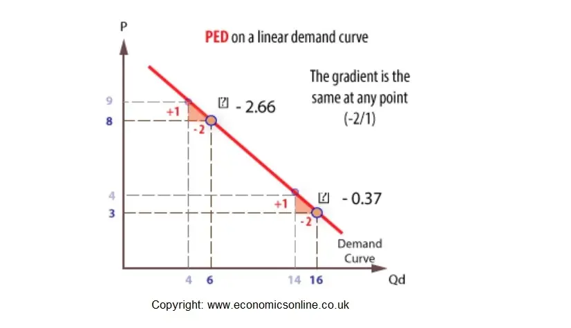
This graph illustrates that on a linear demand curve, elasticity is higher at higher prices (and lower quantities) and lower at lower prices (and higher quantities). In this example, elasticity is -2.66 in the upper region and -0.37 in the lower region.

This happens because elasticity depends on the ratio $P / Q$ . As we move down the demand curve, price $P$ falls and quantity $Q$ rises, so the ratio $P / Q$ continuously decreases. Consequently, the absolute value of elasticity is high at the top of the curve and low at the bottom.

To solidify your understanding of both methods, the following document provides a concise summary of the formulas and a worked example comparing them.

[PDF] Economics 101

This handout from a University of Chicago course provides a compact reference for both elasticity formulas and applies them to the same problem.

Please read page 1 of the document. First, review the formulas provided for Point and Arc Elasticity. Note that "Arc Elasticity" is another name for the midpoint method. Next, work through Exercise 1, parts (a) and (b). Here, the author calculates elasticity for a price change from $15 to $30 using both the simple percentage change method (which they call "Point method" in this context) and the midpoint method. Notice that the two methods give different results (1/3 vs. 3/5). This highlights the importance of the midpoint formula for arc calculations.

Practice Problem

Now it's time to apply what you've learned. Let's solve a typical exam-style problem.

This problem asks you to calculate the price elasticity of demand between points B and C using the Midpoint Method, based on the provided table for snow shovels.

Your task: Calculate the price elasticity of demand as the price changes from point B to point C. Use the midpoint method and provide your answer as an absolute value rounded to two decimal places.

Setup:

Point B: $P_{1} = 11$ , $Q_{1} = 9, 000$
Point C: $P_{2} = 12$ , $Q_{2} = 8, 000$

Apply the midpoint formula:

∣ E_{d} ∣ = \frac{( Q _{2} - Q _{1} ) / (( Q _{1} + Q _{2} ) /2 )}{( P _{2} - P _{1} ) / (( P _{1} + P _{2} ) /2 )}

...

Solution:

∣ E_{d} ∣ = \frac{( 8000 - 9000 ) / (( 9000 + 8000 ) /2 )}{( 12 - 11 ) / (( 11 + 12 ) /2 )}

∣ E_{d} ∣ = \frac{- 1000/ ( 17000/2 )}{1/ ( 23/2 )} = \frac{- 1000/8500}{1/11.5}

∣ E_{d} ∣ = \frac{- 0.1176}{0.0870} \approx ∣ - 1.352∣ \approx 1.35

The price elasticity of demand between points B and C is approximately 1.35.

Conclusion

In this lesson, you've mastered the two primary techniques for calculating price elasticity of demand, a core skill for the CB2 exam and for economic analysis. Your quantitative background allows you to appreciate the distinction between the precision of the point method and the practicality of the midpoint method.

Key Takeaways:

Price elasticity of demand measures the percentage change in quantity demanded for a one percent change in price.
The point elasticity method ( $E_{d} = \frac{d Q}{d P} \cdot \frac{P}{Q}$ ) is used when the demand function is known and you need to find the elasticity at a specific point. It offers calculus-level precision.
The midpoint method ( $E_{d} = \frac{Δ Q / Q _{a v g}}{Δ P / P _{a v g}}$ ) is used to calculate the average elasticity between two distinct price-quantity points. It provides a consistent measure regardless of the direction of the price change.
For a linear demand curve, the slope is constant, but the elasticity is not. Elasticity is typically higher (in absolute value) at higher prices and lower at lower prices.

In our next lesson, we will explore the practical application of these calculations. You will learn how the value of elasticity—specifically, whether demand is elastic ( $∣ E_{d} ∣ > 1$ ), inelastic ( $∣ E_{d} ∣ < 1$ ), or unit elastic ( $∣ E_{d} ∣ = 1$ )—determines what happens to a firm's total revenue when it changes its prices. This relationship is a cornerstone of business pricing strategy.

Recommended resources