Calculating Opportunity Cost

1. Defining Opportunity Cost: More Than Just Money

At its core, economics is the study of how people make choices under conditions of scarcity. Because resources like time, money, and materials are limited, every decision to use a resource for one purpose means giving up the chance to use it for another.

The opportunity cost of a chosen option is the value of the next-best alternative that was forgone.

It's crucial to emphasize "next-best." If you have three choices—A, B, and C—and you choose A, its opportunity cost isn't the combined value of B and C. If B was your second preference, the opportunity cost of choosing A is simply the value you would have derived from B.

To calculate opportunity cost accurately, we must consider two types of costs:

• Explicit Costs: These are the direct, out-of-pocket monetary payments made for a choice. Examples include tuition fees, the price of a movie ticket, or the cost of gasoline. These are typically easy to identify and measure.
• Implicit Costs: These represent the value of resources that are used but not paid for directly in money. The most common implicit cost is the value of your time, often measured by the income you could have earned by working instead. Another example is the forgone interest you could have earned on money you spend today.

A common pitfall is to include sunk costs in the calculation. A sunk cost is an expense that has already been incurred and cannot be recovered. Since it's unavoidable regardless of the decision you make now, it is irrelevant to the opportunity cost of a future choice.

2. Calculating Opportunity Cost: Worked Examples

Your preference for quantitative problem-solving will be particularly useful here. Let's work through some numerical examples to make these concepts concrete. The following problem set from UC Davis provides excellent scenarios for calculation.

Let's break down the logic from the problem set. To find the full opportunity cost, we sum the explicit and implicit costs for each option.

Opportunity Cost of Train:

• Explicit Costs: $25 (ticket)
• Implicit Costs: 2 hours × $20/hour = $40 (forgone wages)
• Total Opportunity Cost = $25 + $40 = $65

Opportunity Cost of Car:

• Explicit Costs: $10 (gas) + $4 (tolls) + ($0.20/mile × 75 miles) = $10 + $4 + $15 = $29
• Implicit Costs: 1.5 hours × $20/hour = $30 (forgone wages)
• Total Opportunity Cost = $29 + $30 = $59

Comparing the two, the opportunity cost of driving ($59) is lower than taking the train ($65). A purely rational economic agent would choose to drive. Notice how the calculation for the car includes vehicle depreciation. This is an explicit cost, albeit not one paid at the pump. The implicit cost of your time, valued at your hourly wage, is what makes the calculation complete.

3. Broadening the Application

The concept of opportunity cost applies to virtually any decision. The following video runs through a series of quick-fire test questions that illustrate this versatility.

The last example in the video is particularly insightful. A government price ceiling on gasoline lowers the explicit cost, but the resulting shortage creates long lines. The full opportunity cost must include the value of the time wasted waiting.

• Situation 1 (No Price Ceiling):

  • Explicit Cost: 20 gallons × $5/gallon = $100
  • Implicit Cost (Time): $0
  • Total Opportunity Cost = $100

• Situation 2 (With Price Ceiling):

  • Explicit Cost: 20 gallons × $4/gallon = $80
  • Implicit Cost (Time): 2 hours × $20/hour = $40
  • Total Opportunity Cost = $80 + $40 = $120

This demonstrates that the seemingly "cheaper" option actually has a higher opportunity cost. This kind of counter-intuitive result is why a disciplined, quantitative approach to opportunity cost is so powerful.

4. Opportunity Cost in Production

The same logic applies to production decisions made by firms or entire countries. When a producer decides to make one good, they are giving up the ability to use those resources (labor, machinery, raw materials) to make something else.

Consider the following tables, which show the production possibilities for two countries, A and B, who can produce either cars or jetpacks.

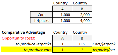
Let's calculate the opportunity costs from the top table.

• Country A: To produce 1,000 cars, it must give up producing 1,000 jetpacks. The opportunity cost of 1 car is therefore $\frac{1000\text{ jetpacks}}{1000\text{ cars}}=1\text{ jetpack per car}$. Conversely, the opportunity cost of 1 jetpack is 1 car.
• Country B: To produce 2,000 cars, it must give up 4,000 jetpacks. The opportunity cost of 1 car is $\frac{4000\text{ jetpacks}}{2000\text{ cars}}=2\text{ jetpacks per car}$. Conversely, the opportunity cost of 1 jetpack is $\frac{2000\text{ cars}}{4000\text{ jetpacks}}=0.5\text{ cars per jetpack}$.

These calculations are summarized in the bottom table. This simple ratio calculation is the foundation for understanding production trade-offs and, as we'll see later in the course, the basis for international trade.

Conclusion

In this lesson, we have moved from a simple idea of cost to a rigorous, analytical framework. By learning to calculate opportunity cost, you can now quantify the trade-offs inherent in any decision.

Key Takeaways:

• Opportunity Cost is the value of the single next-best alternative forgone.
• The calculation must include both explicit costs (direct payments) and implicit costs (forgone value, especially time).
• Sunk costs are past, unrecoverable expenses and are irrelevant to calculating the opportunity cost of a future decision.
• A lower monetary price does not always mean a lower opportunity cost, as other implicit costs may arise.
• The principle applies universally, from an individual's choice of commute to a nation's choice of what goods to produce.

This ability to calculate trade-offs is a cornerstone of economic analysis. In our next lesson, we will expand on this by visualizing the production trade-offs for an entire economy. We will learn to plot a production possibility frontier (PPF) and use its slope to represent opportunity cost graphically.