Deriving AS-AD from IS-LM

Deriving the Aggregate Demand (AD) Curve

The Aggregate Demand curve illustrates the relationship between the overall price level ($P$) in an economy and the corresponding quantity of output ($Y$) for which the goods and money markets are simultaneously in equilibrium. In essence, for every possible price level, there is a unique IS-LM equilibrium, and the AD curve plots these ($P,Y$) pairs.

The Graphical Derivation

Let's begin by understanding the logic visually. The key link between the price level and the IS-LM model is the real money supply, $M/P$. While the IS curve, which represents goods market equilibrium, does not directly depend on $P$, the LM curve most certainly does.

• IS Curve: $Y=C(Y-T)+I(r)+G$ (unaffected by $P$)
• LM Curve: $M/P=L(r,Y)$ (shifts when $P$ changes)

Consider what happens when the price level increases. For a fixed nominal money supply $M$, a higher $P$ reduces the real money supply $M/P$. This creates an excess demand for real money balances at the initial interest rate and income level. To restore equilibrium in the money market, the interest rate must rise, which corresponds to a leftward (or upward) shift of the LM curve.

The following diagram illustrates this process.

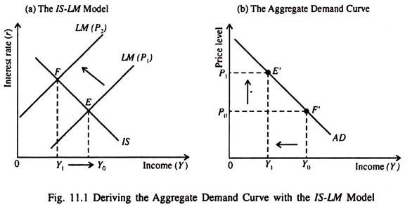
The intuition is straightforward:

1. A higher price level $P$ reduces the real money supply $M/P$.
2. This shifts the LM curve to the left, raising the equilibrium interest rate $r$.
3. The higher interest rate reduces investment spending $I(r)$.
4. Lower investment leads to a lower equilibrium output $Y$.

The result is a negative relationship between the price level and equilibrium output, which is why the AD curve slopes downward.

The Algebraic Derivation

Given your background, you'll appreciate the formal derivation. We derive the AD curve by solving the IS and LM equations for $Y$ as a function of $P$, eliminating the interest rate $r$.

The following reading provides a rigorous algebraic derivation of the AD curve's slope and also discusses factors that cause the curve to shift.

To solidify your understanding, let's work through a numerical example. This is precisely the kind of problem you might encounter on your exam.

Constructing the Aggregate Supply (AS) Curve

The AD curve tells us the equilibrium output for any given price level. However, it doesn't tell us what the price level will actually be. For that, we need to model the supply side of the economy. The Aggregate Supply (AS) curve shows the total quantity of goods and services that firms plan to produce and sell at each price level. It is crucial to distinguish between the long run and the short run.

The Long-Run Aggregate Supply (LRAS) Curve

In macroeconomics, the long run is a period long enough for all prices, including nominal wages, to fully adjust to changes in the economy. In this long-run equilibrium, the economy's output of goods and services is determined by its endowments of capital ($K$) and labor ($L$), and the available production technology ($A$).

This level of output is often called the potential output or full-employment output. Because this potential output $\bar{Y}$ does not depend on the price level, the Long-Run Aggregate Supply (LRAS) curve is a vertical line at $Y=\bar{Y}$. Any changes in the price level are met with proportional changes in wages and other input costs, leaving the real incentives for production unchanged.

The Short-Run Aggregate Supply (SRAS) Curve

The short run is a period during which some prices are "sticky" or inflexible. The assumption of sticky prices is a cornerstone of Keynesian economics and explains why output can deviate from its potential level. The most common explanation for an upward-sloping SRAS curve is the sticky-wage theory.

The Sticky-Wage Model:
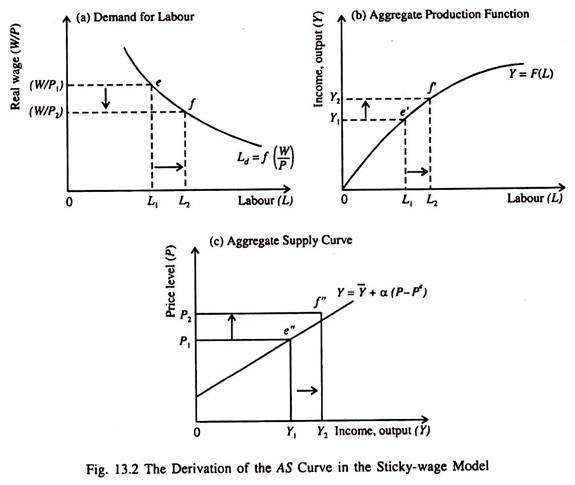
This model assumes that nominal wages ($W$) are fixed in the short run, often due to labor contracts or social norms.

1. The real wage is $W/P$.
2. If the price level $P$ rises, the real wage $W/P$ falls.
3. With a lower real wage, labor becomes cheaper for firms.
4. Firms hire more labor.
5. Increased employment leads to increased output.

This creates a positive relationship between the price level and the quantity of output supplied in the short run. Therefore, the SRAS curve is upward-sloping. The following image neatly illustrates this causal chain.

The reading from the University of Victoria provides more detail on the different models of aggregate supply.

By bringing AD and AS together, we create a model that can determine both the equilibrium price level and the equilibrium level of output simultaneously.

Conclusion

In this lesson, we bridged the gap between our short-run IS-LM analysis and a more complete macroeconomic model. By allowing the price level to vary, we derived the Aggregate Demand curve and explored the theories behind the shape of the Aggregate Supply curve.

Key Takeaways:

• The Aggregate Demand (AD) curve is derived from the IS-LM model. It is downward-sloping because a higher price level reduces real money balances, which raises the interest rate and reduces investment and equilibrium output.
• The equation for the AD curve can be found algebraically by solving the IS and LM equations for output ($Y$) as a function of the price level ($P$).
• The Long-Run Aggregate Supply (LRAS) curve is vertical at the economy's potential output ($\bar{Y}$). In the long run, output is determined by real factors of production, not the price level.
• The Short-Run Aggregate Supply (SRAS) curve is upward-sloping, most commonly explained by the sticky-wage theory. When nominal wages are fixed, a higher price level lowers real wages, stimulating hiring and production.

In our next lesson, we will combine these curves into the full AD-AS model. This powerful framework will allow us to analyze how various economic events—such as changes in government policy, shifts in consumer confidence, or supply-side shocks like an oil price increase—affect both output and inflation in the short and long run.