AD-AS Model: Shocks to Output and Price Level

Introduction

Welcome to the next lesson in our study of macroeconomic models. In the previous lesson, we assembled the essential components of our analytical toolkit: the Aggregate Demand (AD) curve, derived from IS-LM equilibrium, and both the short-run (SRAS) and long-run (LRAS) Aggregate Supply curves. You now understand the theoretical underpinnings of each curve and why they have their respective slopes.

Today, we put this model to work. The primary purpose of the AD-AS framework is to analyze how the economy responds to various shocks—sudden, unexpected events that cause fluctuations in output and the price level. This lesson focuses on fulfilling the learning outcome: "Use the AD-AS model to calculate the effects of demand-side and supply-side shocks on output and the price level." We will trace the economy's path from an initial long-run equilibrium, through the short-run disruption caused by a shock, to its eventual return to a new long-run equilibrium. This analytical process is fundamental to understanding business cycles and forms the basis for the policy debates we will explore next.

The Dynamics of Economic Shocks

Our analysis will always follow a structured, three-step process:

Initial State: We begin by assuming the economy is in a long-run equilibrium, where the AD, SRAS, and LRAS curves all intersect at a single point. Here, output is at its potential level ( $Y = Y ˉ$ ), and the price level is stable.
The Shock: An event shifts either the AD curve or the SRAS curve.
Short-Run Impact: We identify the new short-run equilibrium at the intersection of the new AD (or SRAS) curve and the original SRAS (or AD) curve.
Long-Run Adjustment: We analyze how price expectations adjust, shifting the SRAS curve until the economy returns to a long-run equilibrium on the LRAS curve.

1. Analyzing Aggregate Demand Shocks

Aggregate demand shocks are events that cause households, firms, or the government to change their spending plans at a given price level. These shocks shift the AD curve.

A Negative Demand Shock: The Onset of a Recession

Let's consider a common scenario: a wave of pessimism sweeps the economy. Consumers, worried about the future, cut back on spending, and firms, anticipating lower sales, postpone investment. This is a negative shock to aggregate demand.

The following video provides an excellent walkthrough of this entire process. As you watch, pay close attention to the sequence of events: the initial shift, the short-run outcome, and the long-run self-correcting mechanism.

Chapter 33: Aggregate Demand and Aggregate Supply

This segment from Dr. Azevedo's "Chapter 33" video demonstrates how the economy responds to a shift in aggregate demand.

Watch the section explaining a decrease in aggregate demand, from this example. The lecturer uses a clear, step-by-step graphical analysis to trace the effects from the initial equilibrium (point A) to the short-run recession (point B) and finally to the new long-run equilibrium (point C).

To formalize what you've just seen, let's analyze the standard AD-AS diagram for a negative demand shock.

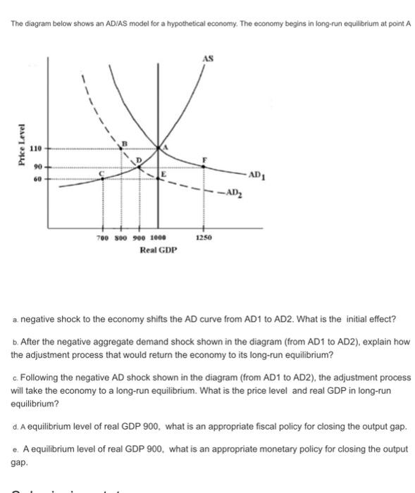
This diagram shows an economy initially in long-run equilibrium at point A, where AD₁, SRAS, and LRAS intersect. A negative shock shifts aggregate demand to AD₂.

Let's break down the effects shown in the diagram:

The Shock: The AD curve shifts left from $A D_{1}$ to $A D_{2}$ .
Short-Run Equilibrium: The economy moves along the initial SRAS curve to point D. At this point, real GDP has fallen from 1000 to 900, and the price level has dropped from 110 to 90. The economy is in a recession, as output is below its long-run potential. The fall in output implies a rise in unemployment.
Long-Run Adjustment: At point D, the price level (90) is lower than what was expected. Over time, these lower price expectations (along with higher unemployment putting downward pressure on wages) cause production costs to fall. This shifts the SRAS curve to the right. This adjustment continues until the SRAS curve intersects the new aggregate demand curve ( $A D_{2}$ ) at a point on the LRAS curve. In the diagram, this would be a point like C, where output has returned to its potential of 1000, but at an even lower price level of 60.

The economy has a self-correcting mechanism. In the case of a demand-driven recession, falling prices and wages eventually restore the economy to full employment, albeit at a lower overall price level.

A positive demand shock (e.g., a stock market boom or an increase in government spending) works in the opposite direction. The AD curve shifts right, leading to a short-run boom (output above potential, higher prices). Over time, rising wage demands shift the SRAS curve left, returning the economy to its potential output level but at a permanently higher price level.

2. Analyzing Aggregate Supply Shocks

Aggregate supply shocks are events that change firms' costs of production, shifting the SRAS curve. The LRAS curve may also shift if the shock is permanent (e.g., a natural disaster that destroys capital stock), but we will focus on temporary shocks that only affect the SRAS curve.

An Adverse Supply Shock: Stagflation

Consider a classic example: a sharp increase in the price of oil. Since oil is a key input for many industries, this raises production costs across the economy.

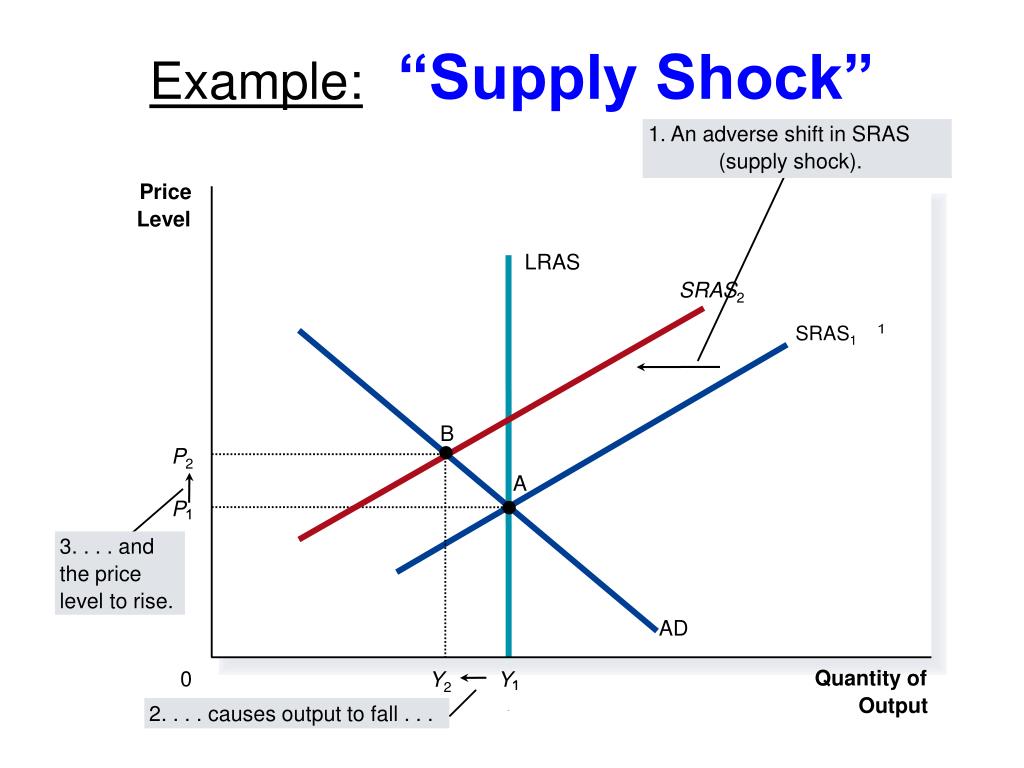
This diagram illustrates an adverse supply shock. The economy starts at point A. A sudden increase in production costs shifts the short-run aggregate supply curve leftward from SRAS₁ to SRAS₂.

The Shock: The SRAS curve shifts left from $S R A S_{1}$ to $S R A S_{2}$ .
Short-Run Equilibrium: The economy moves along the AD curve to a new equilibrium at point B.
Outcome: The result is a uniquely painful combination:
- Output falls from $Y_{1}$ to $Y_{2}$ (a recession).
- The price level rises from $P_{1}$ to $P_{2}$ (inflation).

This phenomenon of falling output combined with rising prices is called stagflation. The following video segment explains this scenario and the difficult policy choices it creates.

Chapter 33: Aggregate Demand and Aggregate Supply

This part of the video analyzes the consequences of a negative shift in short-run aggregate supply.

Please watch the section covering shifts in aggregate supply, from this analysis. Focus on the description of stagflation and the policy dilemma that policymakers face.

As the video highlights, policymakers face a trade-off. They can:

Do nothing and wait for the self-correcting mechanism. The high unemployment from the recession will eventually put downward pressure on wages, shifting the SRAS curve back towards its original position.
Intervene by using fiscal or monetary policy to increase aggregate demand (shift AD to the right). This can restore output to its potential level more quickly but at the cost of "accommodating" the supply shock, leading to a permanently higher price level.

3. Quantitative Application of the AD-AS Model

Your analytical background will be particularly useful here. We can represent the AD-AS model as a system of equations and solve for the equilibrium values of output and inflation/price level. This allows us to precisely calculate the impact of shocks.

The following resource presents a slightly more advanced version of the model where the vertical axis is the inflation rate ( $π$ ) rather than the price level ( $P$ ), but the underlying logic is identical. It provides an excellent numerical problem that is directly relevant to your exam preparation.

[PDF] Macroeconomics - Week 8: The Aggregate Demand & Supply Model

This document contains a series of exercises applying the AD-AS framework. We will focus on a specific numerical problem.

Please navigate to "EXERCISE 5. A DEMAND SHOCK" on page 19. First, review the setup. You are given equations for the AD and AS curves and values for all parameters. AD: Y = m \cdot A - m \cdot \phi \cdot (r + \lambda\pi) AS: \pi = \pi^e + \gamma (Y - Y^P) + \rho Work through part (a). The solution on page 21 shows that by substituting the given values, you can solve this system of two equations for the two unknowns, Y and \pi. The solution is Y = 14 and \pi = 2\%. Read through parts (b) and (c). They establish that since equilibrium output Y equals potential output Y^P, the economy is in a long-run equilibrium. Finally, study part (d) carefully. A demand shock is introduced: government spending increases by 0.2 trillion dollars, which increases the parameter A. The explanation and graph on page 25 show the full dynamic adjustment: Short-run: A new short-run equilibrium with a boom (Y_1 = 14.2 > Y^P) and higher inflation (\pi_1 = 3\%). Long-run adjustment: The boom triggers higher inflation expectations (\pi^e rises), which shifts the AS curve upward (leftward). New Long-run equilibrium: The economy returns to potential output (Y_2 = Y^P = 14), but with a permanently higher inflation rate of \pi_2^* = 4\%. This exercise is a perfect example of how to "calculate the effects of demand-side...shocks," directly matching our learning outcome.

Conclusion

Today we have moved from theory to application, using the AD-AS model as a powerful tool for analyzing economic fluctuations. You have learned to trace the short-run and long-run consequences of both demand-side and supply-side shocks, not just graphically but also through quantitative analysis.

Key Takeaways:

Demand Shocks: A negative AD shock leads to a recession with falling prices. A positive AD shock leads to a boom with rising prices. In both cases, the economy's self-correcting mechanism eventually returns output to its potential level ( $Y ˉ$ ), but the price level is permanently changed.
Supply Shocks: An adverse SRAS shock is particularly problematic, causing stagflation—a recession combined with inflation. This presents a difficult trade-off for policymakers.
Calculation: The effects of shocks can be calculated precisely by defining the AD and AS curves as a system of equations and solving for equilibrium output ( $Y$ ) and the price level ( $P$ ) or inflation rate ( $π$ ).

In our next lesson, we will build directly on this foundation. Having seen how shocks can push the economy away from its desired state, we will delve into the debates surrounding the use of policy to manage these fluctuations. We will calculate fiscal multipliers and compare the effectiveness of different policy interventions, as viewed by competing schools of macroeconomic thought.

Recommended resources