IS-LM Model: Fiscal and Monetary Policy Impacts

Fiscal Policy and the IS-LM Model

Fiscal policy refers to the government's use of its spending and taxation powers to influence the economy. These actions directly impact the components of aggregate demand and therefore shift the IS curve.

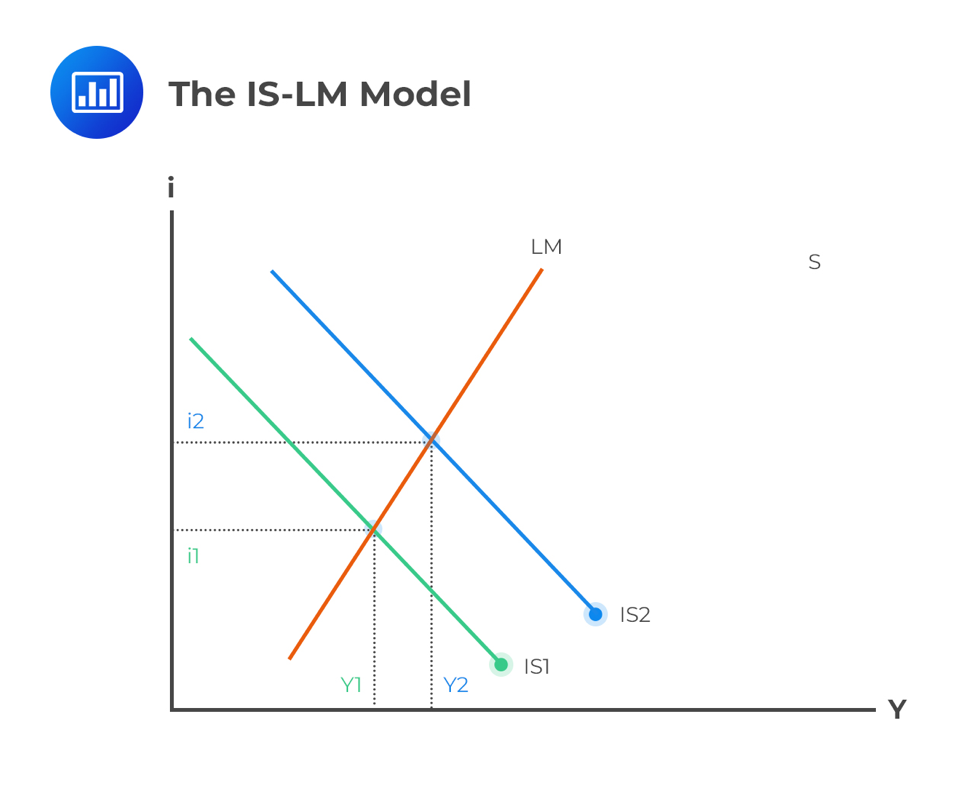
• Expansionary Fiscal Policy: An increase in government spending (G) or a decrease in taxes (T) increases aggregate demand at any given interest rate. This shifts the IS curve to the right.
• Contractionary Fiscal Policy: A decrease in government spending (G) or an increase in taxes (T) reduces aggregate demand. This shifts the IS curve to the left.

The LM curve, which represents money market equilibrium, is not directly affected by G or T. Therefore, a fiscal policy action results in a movement along the LM curve to a new equilibrium.

Graphical Analysis

Let's first visualize how a fiscal contraction works. The following video from MIT OpenCourseWare explains the logic behind the IS curve shift and the adjustment to the new equilibrium. The lecturer also introduces a modern simplification where the central bank targets the interest rate, making the LM curve horizontal. This means fiscal policy changes output without affecting the interest rate, a point we will return to later.

The graphical effect of an expansionary fiscal policy (e.g., an increase in G) is the opposite. The IS curve shifts to the right, leading to a higher equilibrium income and, in the classic model with an upward-sloping LM curve, a higher interest rate.

Quantitative Analysis: The Fiscal Multiplier

While the graph shows the direction of change, your goal is to calculate the precise magnitude. To do this, we can derive the fiscal policy multiplier, which tells us by how much equilibrium income changes for each unit change in government spending.

The following resource derives this multiplier using Cramer's rule, a systematic way to solve systems of linear equations. Given your background in statistics and quantitative methods, you should find this approach both rigorous and efficient.

The term $\frac{d_1{b}_2}{d_2}$ in the denominator is crucial. It represents the "crowding out" effect. A simple Keynesian multiplier would just be $\frac{1}{1-c_1-b_1}$. However, in the IS-LM model, the increase in income raises money demand, which pushes up the interest rate. This higher interest rate reduces investment (the $b_2$ term), partially offsetting the initial expansion. This makes the IS-LM fiscal multiplier smaller than the simple Keynesian multiplier.

Monetary Policy and the IS-LM Model

Monetary policy is conducted by the central bank and involves managing the money supply and interest rates. In our model, this directly affects the LM curve.

• Expansionary Monetary Policy: An increase in the money supply (M) shifts the LM curve to the right (or down). This means that for any given level of income, the interest rate that clears the money market is now lower.
• Contractionary Monetary Policy: A decrease in the money supply (M) shifts the LM curve to the left (or up), leading to a higher equilibrium interest rate for any given level of income.

The IS curve is not directly affected by a change in the money supply, so monetary policy causes a movement along the IS curve.

Graphical Analysis

Quantitative Analysis: A Worked Example

Let's return to the numerical problem from our previous lesson and see how a change in monetary policy affects the equilibrium. The following video calculates the new equilibrium after the money supply increases. This will solidify your ability to re-calculate the equilibrium after a policy shock.

Quantitative Analysis: The Monetary Multiplier

Just as with fiscal policy, we can derive a general multiplier for monetary policy. This tells us how much equilibrium income changes for a change in the real money supply. The derivation is analogous to the fiscal multiplier.

Your Turn: Practice Problems

Now, apply these concepts to solve for the effects of policy changes in a new scenario.

Consider an economy described by the following equations:

• Consumption: $C=200+0.25(Y–T)$
• Investment: $I=150+0.25Y–1000i$
• Government Spending: $G=250$
• Taxes: $T=200$
• Money Demand: $M^d=2Y–8000i$
• The price level P is fixed at 1.

From the previous lesson, you know the initial equilibrium for this economy is $Y^{\ast }=1000$, $i^{\ast }=0.05$ (or 5%), and the initial money supply is $M^{\ast }=1600$.

Problem 1: Monetary Policy
Suppose the central bank cuts the interest rate to 3%.
a. What is the new equilibrium output $Y$?
b. What level of money supply ($M$) is required to achieve this?
c. What are the new equilibrium values of consumption $C$ and investment $I$?

Problem 2: Fiscal Policy
Return to the initial equilibrium ($Y=1000,i=0.05$). Now, suppose government spending increases to G = 400. The central bank acts to keep the interest rate constant at 5%.
a. What is the new equilibrium output $Y$?
b. What are the new values of consumption $C$ and investment $I$?
c. What money supply ($M$) is now required to hold the interest rate at 5%?

Self-Check Solutions:
Problem 1:
a. $Y=1040$
b. $M=1840$
c. $C=410$, $I=380$ (Note: C+I+G = 410+380+250 = 1040)

Problem 2:
a. $Y=1300$
b. $C=475$, $I=425$
c. $M=2200$

These problems are adapted from the problem set by Pascal Michaillat (resource_id="[LINK](https://pascalmichaillat.org/y31.pdf)"), which you can use for further practice if you wish.

Conclusion

In this lesson, we have moved from simply solving the IS-LM model to actively using it for policy analysis. You have seen how fiscal and monetary policies shift the IS and LM curves, respectively, and you have calculated the resulting changes in equilibrium income and interest rate.

Key Takeaways:

• Fiscal policy (G, T) shifts the IS curve and causes a movement along the LM curve. Its effect on income is captured by the fiscal multiplier, which is dampened by the crowding out of investment.
• Monetary policy (M) shifts the LM curve and causes a movement along the IS curve. Its effect is transmitted through the interest rate's influence on investment.
• By deriving and applying policy multipliers, or by re-solving the system of equations, we can precisely quantify the macroeconomic impact of government and central bank actions.

So far, our analysis has assumed a fixed price level. This is a reasonable assumption for the very short run. In our next lesson, we will relax this assumption. We will use the IS-LM model to derive the Aggregate Demand (AD) curve, which shows the relationship between the overall price level and the equilibrium quantity of output demanded in the economy. This will be a crucial step toward building a more complete model of the macroeconomy.