Quantity Theory of Money and Price Level

The Equation of Exchange

At the heart of the quantity theory is a relationship called the equation of exchange. In its most basic form, it's an identity—a statement that is true by definition. It links the amount of money in an economy to the total value of transactions.

The equation is:

Let's break down each component. The image below provides a quick reference, although it uses $T$ for transactions, which we will soon replace with $Y$ for output.

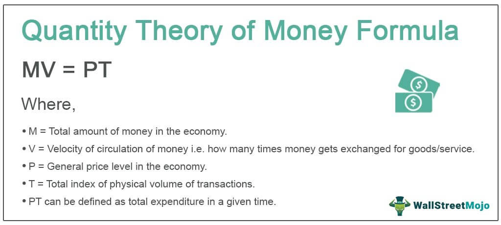
• M (Money Supply): The total amount of money in circulation.
• V (Velocity of Money): The average number of times a unit of money (e.g., a dollar) is spent on final goods and services in a given period. It measures how quickly money circulates through the economy.
• P (Price Level): The average price of all final goods and services produced in the economy (e.g., the GDP deflator).
• Y (Real GDP): The total quantity of all final goods and services produced.

The right side of the equation, $P\times Y$, gives us the Nominal GDP, which is the total dollar value of everything produced. The left side, $M\times V$, represents the total amount of spending in the economy. By definition, total spending must equal the value of what was purchased.

To see how these components are formally defined and linked, the following video provides a concise explanation. It also clarifies why economists often use Real GDP ($Y$) as a practical proxy for the total volume of transactions ($T$), which is much harder to measure.

From an Identity to a Theory

The equation of exchange itself doesn't make any predictions; it's always true. To turn it into a testable theory—the Quantity Theory of Money—we must introduce a few key assumptions about how these variables behave, particularly in the long run.

1. Velocity (V) is stable: The theory assumes that the velocity of money is relatively constant over time. The institutional factors that determine velocity, such as how often people are paid, the efficiency of payment systems (like credit cards and electronic transfers), and general spending habits, do not change quickly. If we assume $V$ is constant, we can denote it as $\bar{V}$.

2. Output (Y) is determined by real factors: In the long run, an economy's ability to produce goods and services ($Y$) is determined by its factors of production (labor, capital, natural resources) and its level of technology. This is the classical dichotomy, which posits that real variables (like output and employment) are not affected by monetary variables (like the money supply) in the long run. This concept is also known as monetary neutrality. We can therefore treat $Y$ as fixed at its potential level, $\bar{Y}$.

With these two assumptions, our equation becomes:

Rearranging to solve for the price level $P$, we get:

Since $\bar{V}$ and $\bar{Y}$ are assumed to be constant, this equation shows a direct, proportional relationship between the money supply ($M$) and the price level ($P$). If the central bank doubles the money supply, the price level will also double. This is the central prediction of the quantity theory: in the long run, changes in the money supply cause proportional changes in the price level.

The following diagram illustrates this relationship from the perspective of the money market. An increase in the money supply (a rightward shift of the vertical money supply curve) reduces the value of money (1/P), which is equivalent to increasing the overall price level (P).

The next segment of the video explains precisely how these assumptions transform the equation into a predictive theory of the price level.

Inflation and Money Growth: The Dynamic Form

For practical analysis, it's often more useful to look at the growth rates of the variables. The quantity equation can be expressed in terms of percentage changes, which, for small changes, is a very good approximation:

Where $\%\Delta M$ is the growth rate of the money supply, $\%\Delta P$ is the growth rate of the price level (i.e., the inflation rate, $\pi$), and so on.

Now, let's re-apply our key assumption from the quantity theory: velocity is constant ($\%\Delta V=0$). The equation simplifies to:

Rearranging to solve for the inflation rate, we get the theory's most powerful result:

This equation provides a clear prediction: the inflation rate is the difference between the growth rate of the money supply and the growth rate of real GDP. If the central bank is printing money faster than the economy is producing new goods and services, the excess money growth will translate directly into inflation. For instance, if the money supply grows by 7% and real GDP grows by 3%, the inflation rate will be approximately 4%.

A key implication is the one-for-one relationship between money growth and inflation. If the growth rate of real GDP is held constant, a 1 percentage point increase in the rate of money growth will cause a 1 percentage point increase in the inflation rate.

This next video segment will walk you through this transformation into growth rates and explain its implications.

Applying the Theory: Calculations

Now, let's put the theory to work by solving a typical exam-style problem. This is where your quantitative skills come into play.

First, let's watch a worked example that uses the inflation equation we just derived, and also connects it back to the Fisher equation (nominal interest rate = real interest rate + inflation), which you've seen in a previous module.

Now, try a similar problem yourself. The following reading contains a "Problems and Applications" section from a standard textbook's solutions manual.

Your calculation should have been:

1. Inflation Rate ($\pi$): $$\pi =\%\Delta M-\%\Delta Y=14\%-5\%=9\%$$
2. Real Interest Rate (r): $$r=\text{Nominal Interest Rate}-\pi =11\%-9\%=2\%$$

This type of calculation is a core application of the theory and is very common in economics exams.

Conclusion

In this lesson, we bridged the gap between changes in the money supply and their long-run effects on the economy. We saw how the simple accounting identity of the equation of exchange transforms into the powerful Quantity Theory of Money with a few key assumptions.

Key Takeaways:

• The equation of exchange, $MV=PY$, is an identity stating that total spending equals the nominal value of output.
• The Quantity Theory of Money assumes stable velocity ($V$) and monetary neutrality (real GDP, $Y$, is unaffected by $M$ in the long run).
• The theory's main prediction is that changes in the money supply lead to proportional changes in the price level.
• In its dynamic form, the theory gives us the inflation equation: $\pi =\%\Delta M-\%\Delta Y$. Inflation is determined by money supply growth in excess of real output growth.

You are now able to analyze and calculate the long-run impact of money supply changes on inflation. This provides the fundamental reason why central banks are so focused on managing the growth of money. In our next lesson, we will turn our attention to the specific monetary policy tools that central banks use to exert this control, such as open market operations and changes to the reserve requirement.