Vector Operations for Asset Prices and Portfolios with NumPy

1. From Python Lists to NumPy Arrays: The "Why"

You're already an expert in using Python lists. So, why do we need another data structure? The answer lies in performance and convenience, two things every developer cares about. In quantitative finance, we often perform mathematical operations on millions of data points. Using standard Python loops for this is far too slow.

NumPy arrays, which we'll use to represent vectors and matrices, are stored in a contiguous block of memory and operations on them are executed by highly optimized, pre-compiled C code. This is a concept known as vectorization.

To get a solid grasp of why this is so critical, let's watch a video that explains the performance benefits from a computer science perspective.

2. Representing Financial Data as Vectors

In linear algebra, a vector is essentially an ordered list of numbers. In Python, we represent this using a 1-dimensional NumPy array. Let's contrast this with a matrix (a 2D array), which we'll cover in the next lesson.

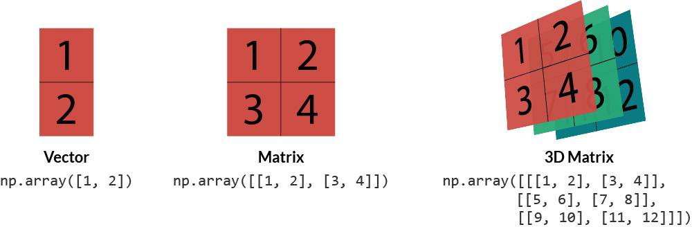
To create a vector representing financial data, we simply convert a Python list into a NumPy array. Let's see how this is done in practice.

Let's imagine a simple portfolio. Suppose you hold:

• 10 shares of Apple (AAPL)
• 5 shares of Microsoft (MSFT)
• 20 shares of NVIDIA (NVDA)

And the current prices are:

• AAPL: $170
• MSFT: $300
• NVDA: $450

We can represent our holdings (quantities) and the asset prices as two distinct vectors:

import numpy as np

# Vector of quantities (number of shares)
quantities = np.array([10, 5, 20])

# Vector of prices
prices = np.array([170.0, 300.0, 450.0])

print("Quantities vector:", quantities)
print("Prices vector:", prices)

3. Vector Operations for Financial Analysis

Now that we have our data in vectors, we can perform calculations.

3.1. Element-Wise Operations

These operations are performed on corresponding elements of two vectors. This is where vectorization shines. For example, to find the profit-and-loss (P&L) for each stock, you might subtract the opening prices from the closing prices.

Here is a code example:

# prices_open and prices_close are vectors
prices_open = np.array([170.0, 300.0, 450.0])
prices_close = np.array([172.5, 298.0, 455.0])

# Calculate the price change for each stock
price_change = prices_close - prices_open
# This is much cleaner than a for loop!

print("Price Change Vector:", price_change)
# Output: Price Change Vector: [ 2.5 -2.   5. ]

# Now, let's use the quantities vector from before
quantities = np.array([10, 5, 20])

# Calculate the P&L for each individual stock
pnl_per_stock = quantities * price_change

print("P&L per Stock Vector:", pnl_per_stock)
# Output: P&L per Stock Vector: [  25.  -10.  100.] 

3.2. Scalar Operations

This involves performing an operation between a vector and a single number (a scalar). For instance, if the entire market jumped 2% due to an economic announcement, you could update all prices in one go:

prices = np.array([170.0, 300.0, 450.0])
market_jump_factor = 1.02 # A 2% increase

new_prices = prices * market_jump_factor

print("New Prices:", np.round(new_prices, 2))
# Output: New Prices: [173.4 306.  459. ]

4. The Dot Product: The Key to Portfolio Calculations

The most important vector operation for portfolio analysis is the dot product. Given two vectors $x$ and $y$, their dot product is the sum of the products of their corresponding elements:
$x\cdot y={\sum }_{i=1}^N{x}_i{y}_i$
This operation is fundamental for calculating weighted sums, such as the total value of a portfolio.

This is exactly what we need to calculate the total value of our portfolio from the quantities and prices vectors.

In NumPy, you can compute the dot product using either np.dot(x, y) or, more modernly, the @ operator (x @ y).

Let's calculate the total value of our portfolio:

quantities = np.array([10, 5, 20])
prices = np.array([170.0, 300.0, 450.0])

# Calculate total portfolio value using the dot product
# (10 * 170) + (5 * 300) + (20 * 450)
portfolio_value = quantities @ prices

print("Total Portfolio Value:", portfolio_value)
# Output: Total Portfolio Value: 12200.0

Another classic use case is calculating the total return of a portfolio when you have a vector of weights and a vector of returns for each asset.

import numpy as np

# Define the vectors
quantities = np.array([100, 50, 10])
prices_open = np.array([50.0, 210.0, 98.0])
prices_close = np.array([52.5, 205.0, 98.5])

# 1. Calculate initial portfolio value
initial_value = quantities @ prices_open
print(f"Initial Portfolio Value: ${initial_value:,.2f}")

# 2. Calculate final portfolio value
final_value = quantities @ prices_close
print(f"Final Portfolio Value: ${final_value:,.2f}")

# 3. Calculate total P&L
total_pnl = final_value - initial_value
print(f"Total Day P&L: ${total_pnl:,.2f}")

# Alternative way to calculate P&L:
# pnl_per_asset = (prices_close - prices_open) * quantities
# total_pnl_alt = np.sum(pnl_per_asset)
# print(f"Total Day P&L (alternative method): ${total_pnl_alt:,.2f}")

Conclusion

In this lesson, we bridged the gap between abstract mathematical concepts and practical, high-performance financial computation. You are now equipped with a foundational skill for any quant developer role.

Key Takeaways:

• Vectors are represented as 1-dimensional NumPy arrays and are ideal for storing ordered financial data like prices, quantities, or weights.
• Vectorization is the practice of applying operations to entire arrays at once, which is significantly faster than using Python loops due to NumPy's optimized C backend.
• Element-wise operations (+, -, *, /) are used to perform calculations between corresponding elements of vectors, such as finding the price change for a list of stocks.
• The dot product (@ or np.dot()) is the essential tool for calculating weighted sums. Its primary applications are calculating a portfolio's total value (quantities @ prices) and its overall return (weights @ returns).

Preview of the Next Lesson:

We've successfully worked with data for a single portfolio at a single point in time using 1D vectors. But what if you want to analyze multiple assets across multiple days, or manage several different portfolios simultaneously? To do that, we need to stack our vectors together to form a matrix (a 2D array). In the next lesson, we will dive into matrix operations, such as multiplication, transposition, and inversion, and see how they enable us to scale our financial analyses.