NumPy Matrix Operations

1. From Vectors to Matrices

A matrix is simply a rectangular grid of numbers, or a collection of vectors of the same size stacked together. In finance, matrices are incredibly useful for organizing data:

• A matrix could hold the daily prices of 500 stocks (rows) over the last 252 trading days (columns).
• It could represent the holdings of 10 different client portfolios (rows) across 30 assets (columns).

We create matrices in NumPy by creating a 2D array, typically from a list of lists.

import numpy as np

# A matrix of prices for 3 stocks over 2 days
# Each inner list is a row (one stock's price history)
prices = np.array([
    [170.0, 172.5],  # Stock A prices
    [300.0, 298.0],  # Stock B prices
    [450.0, 455.0]   # Stock C prices
])

print("Shape of prices matrix:", prices.shape)
# Output: Shape of prices matrix: (3, 2) -> 3 rows, 2 columns

This matrix structure allows us to perform operations across all our data simultaneously, leveraging the power of vectorization we discussed previously.

2. Matrix Transposition

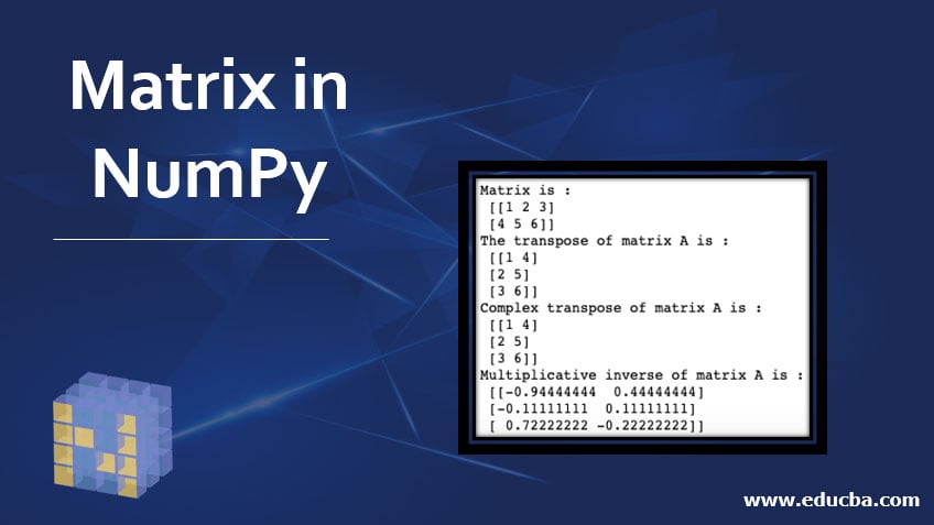
The transpose of a matrix is an operation that flips the matrix over its diagonal, switching the row and column indices. An $m\times n$ matrix becomes an $n\times m$ matrix. This is a fundamental operation in linear algebra, often used to make vectors and matrices conform to the rules of multiplication.

In NumPy, you can transpose a matrix using either the np.transpose() function or the more convenient .T attribute.

Here is a code example to illustrate the concept:

# Our (3, 2) prices matrix from before
prices = np.array([
    [170.0, 172.5],
    [300.0, 298.0],
    [450.0, 455.0]
])

# Transpose it
prices_transposed = prices.T

print("Original shape:", prices.shape)
print("Transposed shape:", prices_transposed.shape)
print("\nTransposed Matrix:\n", prices_transposed)

# Now each row represents a day, and each column a stock.
# [[170.  300.  450. ]  <- Day 1 prices for all stocks
#  [172.5 298.  455. ]] <- Day 2 prices for all stocks

3. Matrix Multiplication: The @ Operator

Matrix multiplication is one of the most important operations in linear algebra. Unlike element-wise multiplication (*), it combines rows from the first matrix with columns from the second matrix.

The Golden Rule: To multiply two matrices, A @ B, the number of columns in matrix A must equal the number of rows in matrix B. If A is (m, n) and B is (n, p), the resulting matrix will be (m, p).

While NumPy has functions like np.dot() and np.matmul(), the modern, preferred syntax introduced in Python 3.5 is the @ operator. It's not just cleaner—it makes complex mathematical formulas significantly more readable, a quality highly valued in professional code.

Let's apply this. Imagine we have two portfolios with different quantities of the same 3 stocks. We can represent this as a (2, 3) matrix. We can then use matrix multiplication with a (3, 1) vector of prices to calculate the total value of each portfolio in a single operation.

# Quantities for two portfolios (2 rows, 3 columns)
quantities = np.array([
    [10, 5, 20],   # Portfolio 1
    [0, 50, 15]    # Portfolio 2
])

# Prices for the three stocks (as a 3x1 column vector)
prices = np.array([
    [170],
    [300],
    [450]
])

# Check dimensions: (2, 3) @ (3, 1) -> (2, 1)
# This is valid!
portfolio_values = quantities @ prices

print("Quantities matrix shape:", quantities.shape)
print("Prices vector shape:", prices.shape)
print("Resulting values shape:", portfolio_values.shape)
print("\nTotal value of each portfolio:\n", portfolio_values)
# [[12200]  <- Value of Portfolio 1
#  [21750]] <- Value of Portfolio 2

4. Matrix Inversion

In regular arithmetic, dividing by a number x is the same as multiplying by its reciprocal 1/x. The inverse of a matrix is a similar concept. The inverse of a square matrix A, denoted as $A^{-1}$, is the matrix that, when multiplied by A, yields the identity matrix I (a matrix with 1s on the diagonal and 0s elsewhere).

$A@A^{-1}=A^{-1}@A=I$

Matrix inversion is crucial for solving systems of linear equations, a common task in finance (e.g., in portfolio optimization).

Key Constraints:

1. Only square matrices (where m = n) can have an inverse.
2. Not all square matrices have an inverse. A matrix without an inverse is called singular. This happens if the matrix's rows or columns are not linearly independent (e.g., one row is a multiple of another).

Here's how you perform an inversion in NumPy:

# A simple 2x2 square matrix
A = np.array([
    [4, 7],
    [2, 6]
])

# Calculate the inverse
A_inv = np.linalg.inv(A)

print("Inverse of A:\n", A_inv)

# Verify by multiplying A by its inverse
# The result should be the 2x2 identity matrix
identity = A @ A_inv

# np.round is used to clean up tiny floating point errors
print("\nA @ A_inv:\n", np.round(identity))
# [[ 1.  0.]
#  [ 0.  1.]]

import numpy as np

# Covariance matrix (2x2)
Sigma = np.array([
    [0.04, 0.018],
    [0.018, 0.09]
])

# Portfolio weights (as a 1D array/row vector)
weights_row = np.array([0.5, 0.5])

import numpy as np

# Given data
Sigma = np.array([
    [0.04, 0.018],
    [0.018, 0.09]
])
weights_row = np.array([0.5, 0.5])

# 1. Reshape the weights vector to be a column vector (2, 1)
weights_col = weights_row.reshape(2, 1)
# The transpose will then be a row vector (1, 2)
weights_transpose = weights_col.T

# You can also use weights_row directly for the transpose part,
# as it already has the correct shape for w^T.

# 2. Calculate variance: (1, 2) @ (2, 2) @ (2, 1) -> (1, 1)
# First part: w^T @ Sigma
part1 = weights_transpose @ Sigma
# Second part: (w^T @ Sigma) @ w
variance = part1 @ weights_col

# The result is a 1x1 matrix, so we extract the scalar value
portfolio_variance = variance[0, 0]

print(f"Weights (column vector):\n{weights_col}\n")
print(f"Portfolio Variance (σ²): {portfolio_variance:.4f}")

# The one-line version is very common in quant code:
# variance_oneline = weights_row @ Sigma @ weights_row
# Note: NumPy is smart about handling the 1D array in this specific case.
# But being explicit with shapes (as done above) is better practice.

Weights (column vector):
[[0.5]
 [0.5]]

Portfolio Variance (σ²): 0.0415

Conclusion

You've now mastered the fundamental matrix operations that form the bedrock of computational finance. These are not just abstract mathematical ideas; they are the tools you will use daily to build, test, and run quantitative models efficiently.

Key Takeaways:

• Matrices (2D NumPy arrays) are used to organize complex datasets, such as the prices of many assets over time.
• Transposition (.T) is a simple but essential operation for reorienting matrices to meet the requirements of linear algebra formulas.
• Matrix Multiplication (@) is the key to combining different sets of data, such as portfolio quantities and asset prices. Its dimension rule ((m, n) @ (n, p) -> (m, p)) is critical to remember.
• Matrix Inversion (np.linalg.inv) is the matrix equivalent of division and is used to solve systems of linear equations, a core task in optimization problems.

Preview of the Next Lesson:

You've already had a sneak peek! We've assembled all the necessary mathematical machinery with vectors and matrices. In the next lesson, "Calculate portfolio returns and volatility using vector and matrix algebra," we will fully formalize the portfolio variance calculation you just practiced and also compute portfolio returns, applying today's operations to solve a concrete and essential finance problem.