Time Value of Money: Present and Future Values

1. The Core Concept: Why Time is Money

Before we get into formulas and code, let's build the intuition. Would you rather have $1,000 today or $1,000 one year from now? You'd almost certainly choose to have it today. Why?

1. Opportunity Cost: You could invest the $1,000 today and have more than $1,000 in a year.
2. Inflation: The purchasing power of $1,000 is likely to be lower in a year due to rising prices.
3. Certainty: Having the money now is a sure thing; a promise of future payment carries risk.

This simple preference is the essence of the time value of money. To formalize this, we need a way to quantify the relationship between money at different points in time.

To get a quick and clear overview of this idea, please watch the first two minutes of the following video.

2. Compounding and Future Value (FV)

If money today is worth more than money in the future, how much more will today's money be worth in the future? This is calculated through compounding. When you invest money, you earn interest. The next period, you earn interest on your initial principal and on the accumulated interest.

The general formula for the Future Value (FV) of a single sum is:

$FV=PV\cdot (1+r{)}^n$

Where:

• $PV$ is the Present Value (the initial amount)
• $r$ is the interest rate per period
• $n$ is the number of periods

Let's continue with the video you started, which now introduces these formulas.

Implementation in Python

As a developer, you'll rarely calculate these values with a pen and paper. Your expertise in Python and numerical libraries is a huge advantage here. Let's see how to calculate future value over several years using NumPy. This approach avoids explicit for loops, which is a core principle in high-performance scientific computing.

The key insight from that code is that instead of looping through each year, you can create an array of growth factors ([1.05, 1.05, ...]) and use np.cumprod() (cumulative product) to get the compounded growth factor at each step ([1.05, 1.1025, ...]). This is far more efficient for large calculations.

import numpy as np

initial_amount = 10000
interest_rate = 0.06
num_years = 5

# Create an array of growth factors for each year
growth_factors = np.full(num_years, 1 + interest_rate)

# Calculate the cumulative growth over the years
cumulative_growth = np.cumprod(growth_factors)

# Calculate the value at the end of each year
yearly_amounts = initial_amount * cumulative_growth

print("Value after each year:", np.round(yearly_amounts, 2))
# Expected output: 
# Value after each year: [10600.  11236.  11910.16 12624.77 13382.26]

3. Discounting and Present Value (PV)

Discounting is the reverse of compounding. It answers the question: "How much is a future cash flow worth to me today?" This is arguably the most important concept in valuation. To value a stock, a bond, or an entire company, you project its future cash flows and "discount" them back to the present.

The formula for Present Value is a simple rearrangement of the FV formula:

$PV=\frac{FV}{(1+r{)}^n}$

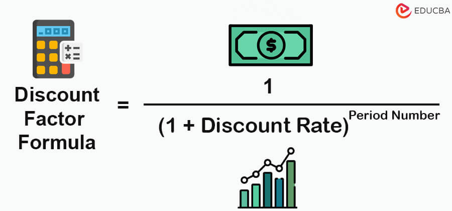
The Discount Factor

You can think of this calculation in two parts. The term $\frac{1}{(1+r{)}^n}$ is called the Discount Factor. It's the value today of $1 received in $n$ periods at a discount rate of $r$.

Once you have the discount factor, calculating the present value is straightforward: $PV=FV\cdot \text{Discount Factor}$.

Application: Discounted Cash Flow (DCF)

A common application is a Discounted Cash Flow (DCF) analysis, where you sum the present values of all expected future cash flows from a project or company to determine its worth today.

This next video shows this in action, introducing the idea of a "discount rate" and applying discount factors to a series of cash flows to find their Net Present Value (NPV).

Implementation in Python

Now, let's implement the discounting of multiple cash flows in Python. Similar to the FV calculation, we can use NumPy to perform this efficiently.

That single line of code is incredibly powerful. Let's break it down:

• free_cash_flow is a NumPy array of future cash flows, e.g., [100, 110, 120].
• np.arange(1, years + 1) creates an array of time periods, e.g., [1, 2, 3].
• The ** operator raises (1 + wacc) to the power of each element in the time period array.
• Finally, the division is performed element-wise.

This is a perfect example of the "vectorized" thinking common in quantitative finance. Instead of writing a loop, you operate on entire arrays at once.

Conclusion

In this lesson, we established the foundational principle of finance: the time value of money. We've seen that compounding calculates a future value, while discounting calculates a present value.

Key Takeaways:

• Money has a time value due to opportunity cost and inflation. A dollar today is worth more than a dollar tomorrow.
• Future Value (FV) is calculated by compounding a present amount forward in time: $FV=PV\cdot (1+r{)}^n$.
• Present Value (PV) is calculated by discounting a future amount back to the present: $PV=\frac{FV}{(1+r{)}^n}$.
• The Discount Factor is the term $\frac{1}{(1+r{)}^n}$, which represents the present value of $1 received in the future.
• As a quant developer, you can use NumPy's vectorized operations to perform these calculations efficiently on entire series of cash flows, which is much faster and cleaner than writing explicit loops.

This concept is the bedrock for almost everything that follows. Whether pricing a bond, valuing an option, or assessing a trading strategy's returns, you are always, in some form, discounting future expectations to make a decision today.

Preview of the Next Lesson:

We got a taste of NumPy's power today. In the next lesson, we will formalize our understanding of the data structures we'll be using. We'll explore how to represent asset prices and portfolio weights as vectors and perform basic vector operations. This is the next essential skill for handling financial data computationally.