Code Embedding with Transformers

Introduction

In our last lesson, we tackled the essential first step of preparing source code for a deep learning model. You learned how to use a code-aware tokenizer, like the one from GraphCodeBERT, to transform a raw string of Python code into a structured format with input_ids and attention_masks. This process converts code into a language that transformer models can understand.

Today, we'll take that tokenized input and perform the main event: feeding it into a pre-trained transformer model to produce a semantic embedding. This is a dense numerical vector that captures the meaning and functionality of the code. By the end of this lesson, you will be able to generate semantic embeddings for code snippets using a pre-trained transformer model.

This is a pivotal moment in our course. Moving from token IDs to embeddings unlocks the ability to have the model "understand" code on a deeper level, far beyond what's possible with the manually-engineered features we used in the classical ML modules.

From Tokens to Meaning: What is an Embedding?

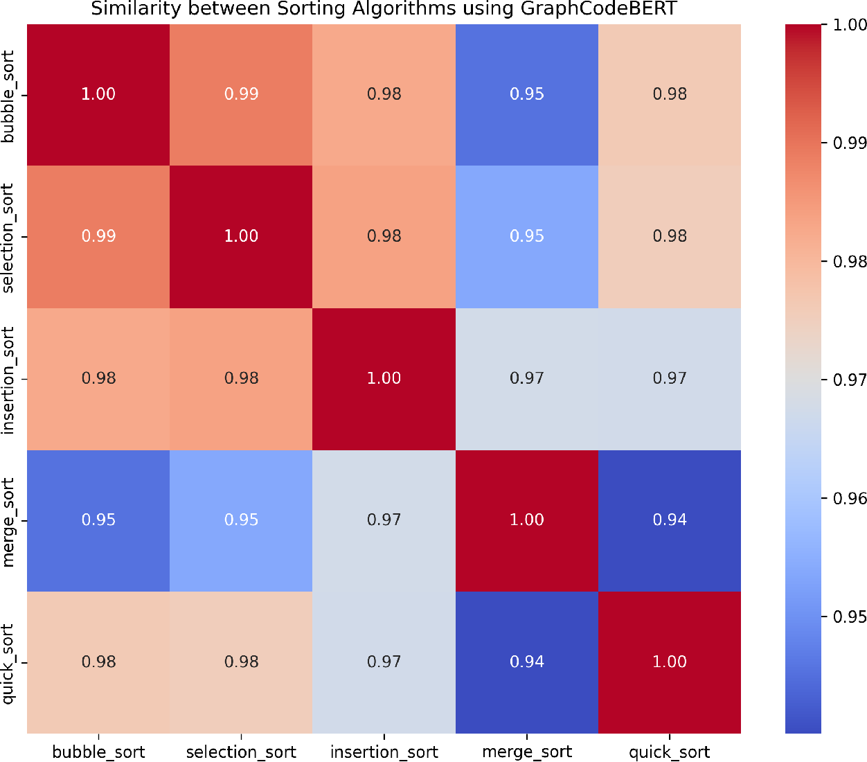
Think of a semantic embedding as a coordinate in a high-dimensional "meaning space." In this space, pieces of code that do similar things—even if written differently—are located close to each other. For example, an embedding for a for loop that sums a list should be near the embedding for a while loop that does the same thing.

How does a model learn to create such meaningful coordinates? Models like CodeBERT and GraphCodeBERT are pre-trained on vast quantities of open-source code from platforms like GitHub. During this pre-training, they learn the statistical relationships between code tokens, syntax structures, and even comments.

Crucially, the most advanced models don't just read code as text. They incorporate its structure.

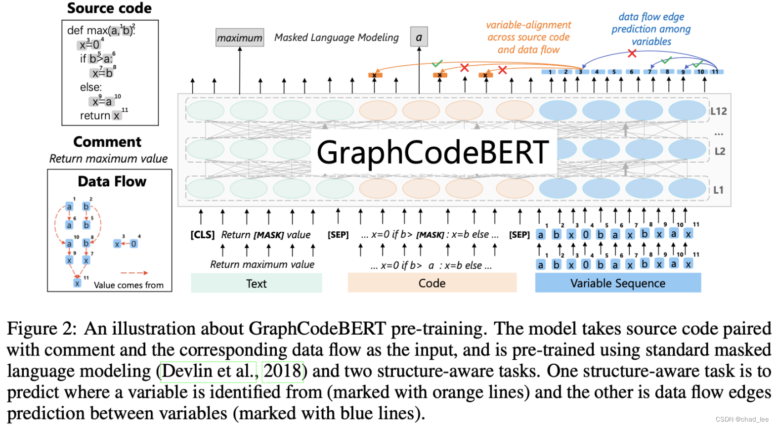
This multi-modal training is what allows the model to generate embeddings that capture not just what the code says, but what it does.

Generating Embeddings with transformers

Let's get practical and extend the code from our previous lesson. You already know how to get the inputs from the tokenizer. Now, we'll load the model itself and pass those inputs to it.

Here is a complete Python script that performs tokenization and model inference.

from transformers import AutoTokenizer, AutoModel
import torch




# 1. Load the same tokenizer and a pre-trained model
# We use AutoModel to get the base transformer without any specific task head.
tokenizer = AutoTokenizer.from_pretrained("microsoft/graphcodebert-base")
model = AutoModel.from_pretrained("microsoft/graphcodebert-base")




# 2. Define our Python function
code = """
def calculate_priority(churn_rate, author_count):



    # High churn by few authors is a red flag
    if churn_rate > 0.8 and author_count <= 2:
        return "High"
    return "Normal"
"""




# 3. Tokenize the code (same as last lesson)
inputs = tokenizer(code, return_tensors="pt", truncation=True, padding="max_length", max_length=64)




# 4. Generate the embeddings
# We use torch.no_grad() because we are not training the model, just doing inference.
with torch.no_grad():
    outputs = model(**inputs)




# 5. Inspect the outputs
last_hidden_state = outputs.last_hidden_state
pooler_output = outputs.pooler_output

print("--- Shape of Last Hidden State ---")
print(last_hidden_state.shape)
print("\n--- Shape of Pooler Output ---")
print(pooler_output.shape)
print("\n--- The Pooler Output Vector (Embedding for the entire snippet) ---")
print(pooler_output)

Running the Code

When you run this script (assuming transformers and torch are installed), you will see output similar to this:

--- Shape of Last Hidden State ---
torch.Size([1, 64, 768])

--- Shape of Pooler Output ---
torch.Size([1, 768])

--- The Pooler Output Vector (Embedding for the entire snippet) ---
tensor([[ 0.0123, -0.1456,  0.9871,  ..., -0.0543,  0.3452,  0.5511]])

Understanding the Output

Let's break down what these tensors represent:

• last_hidden_state: This tensor has the shape (batch_size, sequence_length, hidden_dim), which is (1, 64, 768) in our case. It contains an embedding vector of size 768 for each of the 64 tokens in our input sequence. This is useful when you need to understand the role of individual tokens.
• pooler_output: This tensor has the shape (batch_size, hidden_dim), or (1, 768). It represents an aggregated embedding for the entire code snippet. By convention, this is the last_hidden_state of the special [CLS] token (the first token in the sequence) after being passed through an additional linear layer and activation function.

For many tasks like classification or similarity search on entire functions, the pooler_output is the semantic embedding you will use. You have successfully converted a multi-line code snippet into a single, dense 768-dimensional vector that captures its meaning.

An Alternative: High-Level Abstraction with towhee

While using the transformers library directly gives you maximum control, sometimes you just want to get from code to an embedding as quickly as possible. This aligns with your goal of "learning just enough to get building." The towhee library provides a high-level API for this.

As you can see from the resource, towhee wraps the entire process—tokenization and model inference—into a single "operator." The code ops.code_search.codebert() loads the model and tokenizer behind the scenes. You simply define a pipeline that takes text as input and maps it to an embedding.

This approach is excellent for rapid prototyping and integrating embedding generation into a larger workflow, which will be valuable as you start building your final project.

Conclusion

In this lesson, we completed the journey from raw code to a meaningful numerical representation. You took the token IDs from the previous step and used a pre-trained model to generate semantic embeddings.

Key Takeaways:

• A semantic embedding is a dense vector that represents the meaning of a code snippet, placing similar code close together in a high-dimensional space.
• Pre-trained models like GraphCodeBERT generate powerful embeddings because they are trained not just on code as text, but also on its underlying structure, like data flow.
• Using the transformers library, you can get two main types of embeddings:
  • last_hidden_state: An embedding for every token in the input.
  • pooler_output: A single, aggregated embedding for the entire input sequence, often used for classification or similarity tasks.
• Libraries like towhee offer higher-level abstractions to simplify the embedding generation process into a clean pipeline.

Preview of the Next Lesson:
So, we have these powerful 768-dimensional vectors. What's next? In our next lesson, "Compute semantic similarity between code functions using cosine similarity on their embeddings," we will put them to immediate use. You'll learn how to take two of these vectors and calculate a score that tells you how semantically similar their original code snippets are.