Visualizing Code Embeddings with Dimensionality Reduction

The Challenge: Visualizing High-Dimensional Space

A GraphCodeBERT embedding is a vector with 768 numbers. Our brains are great at visualizing data in two or three dimensions, but we have no intuition for what a 768-dimensional space "looks like." Trying to plot this directly is impossible.

The solution is dimensionality reduction. This is a set of techniques that take high-dimensional data and create a lower-dimensional representation (a "projection" or "embedding") while trying to preserve the most important structural information. Imagine taking a 3D globe and creating a 2D flat map of the world—you lose some information (areas get distorted), but you preserve the relative positions of continents. Dimensionality reduction does the same, but from a much higher starting dimension.

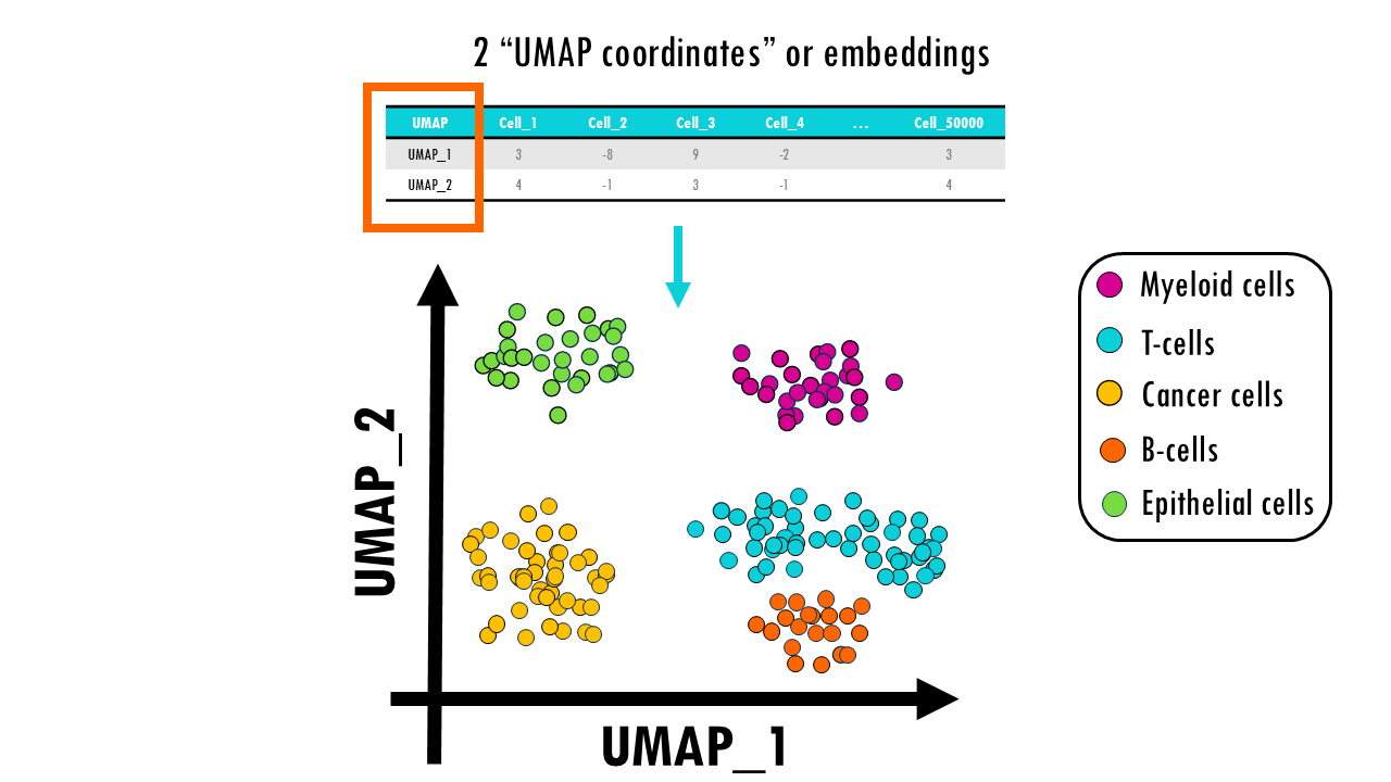
UMAP and t-SNE: Tools for Visualization

Two of the most popular algorithms for this task are t-SNE (t-distributed Stochastic Neighbor Embedding) and UMAP (Uniform Manifold Approximation and Projection). While t-SNE has been a standard for many years, UMAP is a more recent technique that often produces better results.

To understand why UMAP is frequently preferred, let's explore its advantages.

As you've just read, UMAP has two main advantages over t-SNE:

1. Speed: It is significantly faster, which is crucial when working with large datasets.
2. Global Structure Preservation: UMAP does a better job of preserving the large-scale structure of the data. This means that the relative positions of clusters in a UMAP plot are more meaningful than in a t-SNE plot.

For these reasons, we will focus on UMAP for our practical example.

Tuning UMAP for Better Insights

A key part of using UMAP effectively is understanding its main hyperparameters, which control how the algorithm balances local detail against the global picture.

To summarize:

• n_neighbors: Controls the balance between local and global structure.
  • Low values (e.g., 2-5): UMAP will focus on very local structure. You'll see tight, well-defined clusters, but you might lose the "big picture" of how they relate.
  • High values (e.g., 15-50): UMAP will look at a wider neighborhood, giving a better representation of the overall topology of your data, potentially at the cost of blurring smaller, distinct clusters.
• min_dist: Controls how tightly UMAP is allowed to pack points together.
  • Low values (e.g., 0.0-0.1): Creates dense, compact clusters, emphasizing the separation between them.
  • High values (e.g., 0.5-0.99): Points will be more spread out, which can help reveal the internal structure of a cluster but makes them look less clumped.

There are no "correct" settings; the best values depend on your data and what you want to discover. Experimentation is key.

From Theory to Code: Visualizing Code with UMAP

Now, let's put this into practice. We'll write a Python script that builds on our previous work. This time, we'll use a more diverse set of functions to see how they cluster.

First, you'll need to install the necessary libraries. Your transformers, torch, and scikit-learn libraries should already be installed from previous lessons.

pip install umap-learn matplotlib

The following script will:

1. Define a set of Python functions with different functionalities (sorting, string manipulation).
2. Generate a 768-D embedding for each function using GraphCodeBERT.
3. Use UMAP to reduce the dimensionality of these embeddings to 2-D.
4. Use Matplotlib to create a scatter plot of the 2-D results, with labels.

import torch
from transformers import AutoTokenizer, AutoModel
import umap
import matplotlib.pyplot as plt
import numpy as np




# --- 1. Setup Model and Tokenizer (from previous lessons) ---
# Using a specific revision for consistency
tokenizer = AutoTokenizer.from_pretrained("microsoft/graphcodebert-base")
model = AutoModel.from_pretrained("microsoft/graphcodebert-base")




# --- 2. Define a diverse set of Code Snippets ---
code_snippets = {
    "bubble_sort": """
def bubble_sort(arr):
    n = len(arr)
    for i in range(n):
        for j in range(0, n-i-1):
            if arr[j] > arr[j+1]:
                arr[j], arr[j+1] = arr[j+1], arr[j]
    return arr
""",
    "insertion_sort": """
def insertion_sort(arr):
    for i in range(1, len(arr)):
        key = arr[i]
        j = i-1
        while j >=0 and key < arr[j]:
            arr[j+1] = arr[j]
            j -= 1
        arr[j+1] = key
    return arr
""",
    "quick_sort": """
def quick_sort(arr):
    if len(arr) <= 1:
        return arr
    pivot = arr[len(arr) // 2]
    left = [x for x in arr if x < pivot]
    middle = [x for x in arr if x == pivot]
    right = [x for x in arr if x > pivot]
    return quick_sort(left) + middle + quick_sort(right)
""",
    "reverse_string": """
def reverse_string(s):
    return s[::-1]
""",
    "is_palindrome": """
def is_palindrome(s):



    # Check if a string is the same forwards and backwards
    return s == s[::-1]
""",
    "count_chars": """
def count_chars(s):



    # Count occurrences of each character in a string
    counts = {}
    for char in s:
        counts[char] = counts.get(char, 0) + 1
    return counts
"""
}




# --- 3. Generate Embeddings for all Snippets ---
print("Generating embeddings...")
embeddings = []
for code in code_snippets.values():
    inputs = tokenizer(code, return_tensors="pt", truncation=True, padding=True)
    with torch.no_grad():
        outputs = model(**inputs)
    snippet_embedding = outputs.pooler_output.detach().numpy()
    embeddings.append(snippet_embedding)

embeddings_matrix = np.vstack(embeddings)
print(f"Embeddings matrix shape: {embeddings_matrix.shape}")




# --- 4. Apply UMAP for Dimensionality Reduction ---
print("Running UMAP...")
reducer = umap.UMAP(
    n_neighbors=2, # Low value to focus on local structure and forming tight clusters
    min_dist=0.1,  # Pack points closely
    random_state=42 # for reproducibility
)
embedding_2d = reducer.fit_transform(embeddings_matrix)
print(f"2D embedding shape: {embedding_2d.shape}")





# --- 5. Visualize the 2D Embeddings ---
plt.figure(figsize=(12, 8))
plt.scatter(embedding_2d[:, 0], embedding_2d[:, 1], s=100)




# Add labels to each point
for i, name in enumerate(code_snippets.keys()):
    plt.annotate(name, (embedding_2d[i, 0], embedding_2d[i, 1]),
                 xytext=(5, -5), textcoords='offset points')

plt.title('2D UMAP Projection of Code Function Embeddings')
plt.xlabel('UMAP Dimension 1')
plt.ylabel('UMAP Dimension 2')
plt.grid(True)
plt.show()

Interpreting the Results

When you run the code, you will get a 2D scatter plot. The output should look something like this:

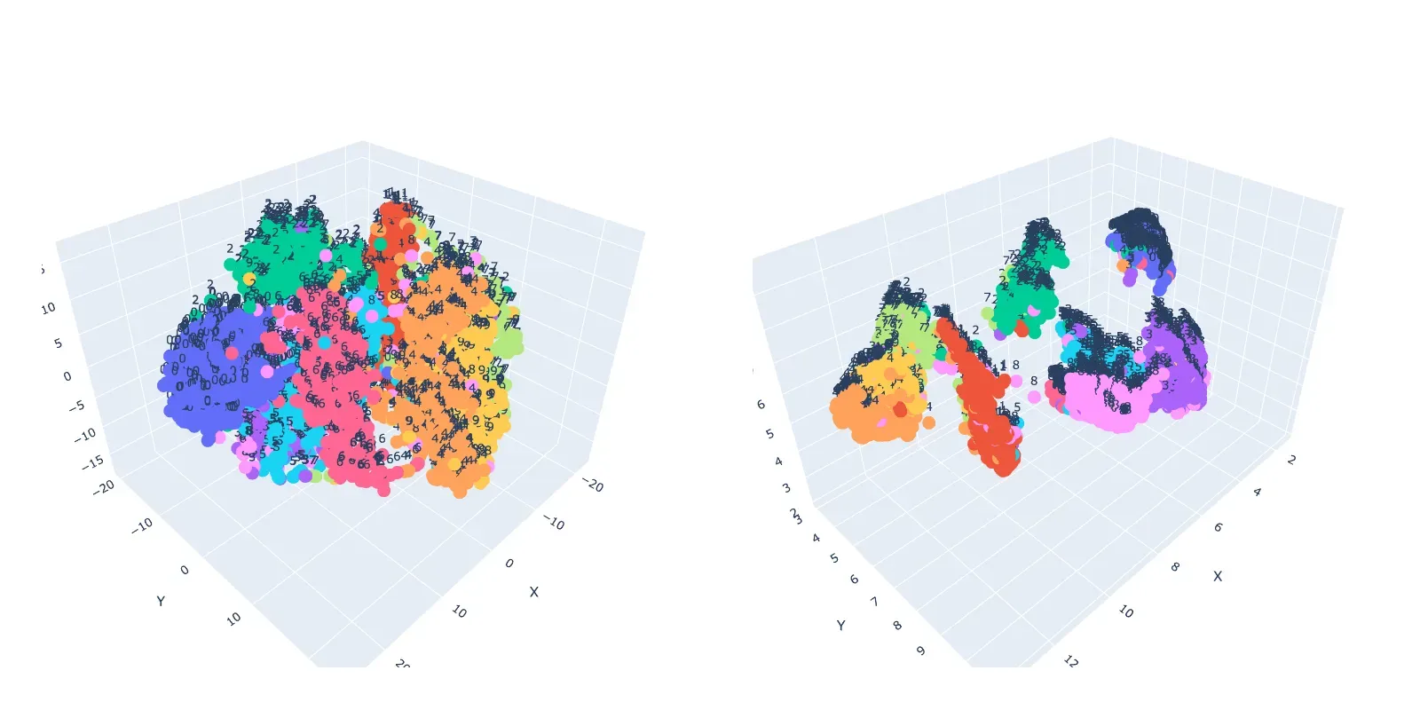
This visual clustering confirms what we intuitively know: the sorting functions are semantically related to each other, and distinct from the string functions. The model, through its embeddings, has captured this functional difference, and UMAP has made it visible to us.

This technique is incredibly powerful for exploring a real-world codebase. You could generate embeddings for all functions in a repository, plot them, and immediately see the main functional modules as distinct clusters.

Finally, while these plots are insightful, it's crucial not to misinterpret them.

Key points to remember:

• Cluster size means nothing. A large-looking cluster isn't necessarily more "varied" than a small one.
• Distances between clusters might not mean anything. Don't assume two clusters that are close together are more related than two that are far apart. UMAP preserves global structure better than t-SNE, but the visual distance is still not a reliable metric.
• Always experiment with hyperparameters. The plot you see is just one possible view of the data.

To see more advanced examples of these visualizations in a research context, you can browse the graphcodebert-interpretability GitHub repository (resource_id=[LINK](https://github.com/jorge-martinez-gil/graphcodebert-interpretability)), which contains numerous comparisons of code snippets visualized with t-SNE, UMAP, and PCA.

Conclusion

In this lesson, you've bridged the gap from abstract, high-dimensional vectors to tangible, visual insights about your code. You now have a powerful exploratory tool at your disposal that can help you understand the architecture of a complex codebase at a glance.

Key Takeaways:

• Dimensionality reduction techniques like UMAP and t-SNE allow us to visualize high-dimensional code embeddings in 2D or 3D.
• UMAP is often preferred for its speed and better preservation of global data structure.
• The n_neighbors and min_dist parameters are critical for tuning the visualization to explore either local detail or global structure.
• Visualizations help us identify clusters of semantically similar code, but we must be careful not to over-interpret cluster size or inter-cluster distances.

Preview of the Next Lesson:
So far in this module, we have learned to create, compare, and visualize code embeddings. We've treated them as objects for exploration. In our next and final lesson of this module, "Use code embeddings as input features for a downstream classification or ranking task," we will put these embeddings to work. You'll learn how to use them as features for standard machine learning models, enabling you to build systems that can automatically classify code (e.g., "is this function buggy?") or rank it for importance.