Ranking Model Evaluation Metrics

Introduction

In our last lesson, we focused on evaluating classification models, like our flaky test detector. You learned that for imbalanced datasets, simple accuracy is misleading and that metrics like precision, recall, and the F1-score give a much clearer picture of performance.

Today, we shift our focus to the second major model type you've built: the learning-to-rank model for technical debt prioritization. This brings us to a new evaluation challenge. For a classifier, a prediction is either right or wrong. For a ranker, the order of the predictions is what matters most. A model that places the most critical technical debt item at rank #1 is far more useful than one that places it at rank #20, even if both models identify the same set of debt items.

This lesson directly addresses the learning outcome: Evaluate ranking model performance using metrics such as nDCG or Mean Average Precision. We will explore two key metrics designed specifically for ranking tasks. By the end, you'll understand how to quantify the "goodness" of an ordered list, a crucial skill for validating your technical debt prioritization tool.

From Classification to Ranking Evaluation

Why can't we just use precision and recall? While we can adapt them (e.g., "Precision at k"), they don't fully capture the essence of ranking. They treat all positions within the top k items equally and typically assume a binary concept of relevance (it's either relevant or it's not).

We need metrics that:

1. Reward placing relevant items higher in the list.
2. Can handle graded levels of relevance (e.g., "critical debt" is more relevant than "minor debt").

Let's start with a metric that builds on the concept of precision but adapts it for ranking.

Mean Average Precision (MAP)

MAP is a popular metric for ranking when you have binary relevance labels (i.e., each item is either relevant or not relevant). It's built on a simpler concept called Average Precision (AP).

• Average Precision (AP) is calculated for a single ranked list. It averages the precision values at each position where a relevant item is found. This rewards models that find relevant items early in the list.
• Mean Average Precision (MAP) is simply the average of the AP scores across all the lists in your test set (e.g., across multiple codebases or sprints for which you're prioritizing debt).

To get a solid grasp of these metrics, let's start with a foundational article.

To make the calculation of Average Precision even more concrete, let's look at a visual breakdown.

MAP is a great metric, but it has one limitation: it assumes binary relevance. What if your technical debt isn't just "debt" or "no debt"? What if you have severity levels like critical, major, and minor? For this, we need a more powerful metric.

Normalized Discounted Cumulative Gain (NDCG)

NDCG is arguably the most popular and powerful ranking metric, precisely because it handles graded relevance.

The name sounds complex, but it's built from three simple ideas:

1. Cumulative Gain (CG): The simplest idea. You just sum up the relevance scores of all items in your ranked list up to position k. A higher score is better. However, it completely ignores the order!
2. Discounted Cumulative Gain (DCG): This is a huge improvement. It still sums the relevance scores, but it "discounts" the score of each item based on its rank. Items at the top get full credit, while items further down have their relevance score reduced by a logarithmic penalty. This directly rewards putting important items first.
3. Normalized Discounted Cumulative Gain (NDCG): There's one last problem. The DCG score isn't easily comparable across lists of different lengths. To fix this, we normalize it. We calculate the DCG of our model's list and divide it by the DCG of a perfectly ranked list (called the Ideal DCG, or IDCG). The result is a score from 0.0 to 1.0, where 1.0 is a perfect ranking.

This step-by-step process is best understood with an example. The following article provides an excellent walkthrough.

The image below provides another excellent visualization of the full NDCG calculation, highlighting the comparison between a predicted ranking and the ideal one.

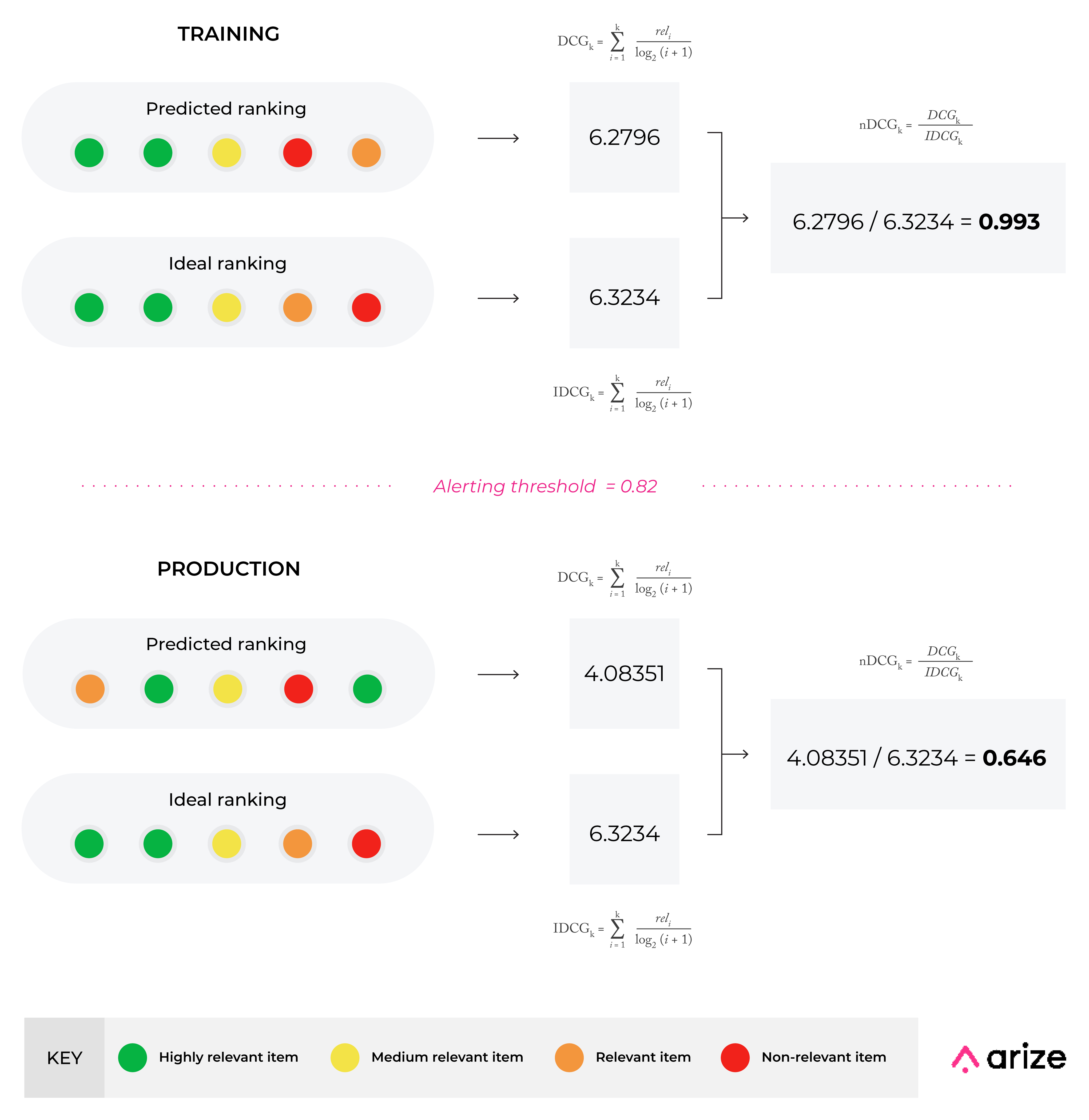
As you can see, NDCG is perfectly suited for your technical debt problem. You could assign relevance scores like:

• 3 for a critical, architecture-level issue.
• 2 for a major bug-inducing pattern.
• 1 for a minor code smell.
• 0 for a non-debt item.

Using NDCG, you could then robustly evaluate how well your model prioritizes the most severe debt.

Practical Implementation with Scikit-learn

Your experience with scikit-learn makes applying these metrics straightforward. The sklearn.metrics module provides functions for both.

• label_ranking_average_precision_score: This calculates the MAP.
• ndcg_score: This calculates the NDCG.

Let's see how to use them. The key is to correctly format the ground truth (y_true) and the model's predicted scores (y_score).

import numpy as np
from sklearn.metrics import label_ranking_average_precision_score, ndcg_score




# --- Scenario: Prioritizing 5 technical debt items ---




# Ground Truth Relevance Scores
# Let's say item 0 is minor, 1 is critical, 2 is none, 3 is major, 4 is minor.
# Relevance: 3=critical, 2=major, 1=minor, 0=none
y_true = np.array([[1, 3, 0, 2, 1]]) 




# Model's Predicted Scores (higher score = higher priority)
# Model A correctly prioritizes the critical item (index 1)
y_score_A = np.array([[0.5, 2.5, 0.1, 1.5, 0.8]]) 




# Model B misses the critical item, prioritizing a major one instead.
y_score_B = np.array([[0.9, 1.2, 0.2, 2.1, 1.5]]) 




# --- Evaluate Model A ---
map_A = label_ranking_average_precision_score(y_true > 0, y_score_A) # MAP binarizes relevance
ndcg_A = ndcg_score(y_true, y_score_A)

print("--- Model A Evaluation ---")
print(f"Model A's Sorted Ranks (by score): {np.argsort(y_score_A[0])[::-1]}")
print(f"True Relevance of Sorted Items: {y_true[0][np.argsort(y_score_A[0])[::-1]]}")
print(f"MAP Score for Model A: {map_A:.4f}")
print(f"NDCG Score for Model A: {ndcg_A:.4f}\n")





# --- Evaluate Model B ---
map_B = label_ranking_average_precision_score(y_true > 0, y_score_B)
ndcg_B = ndcg_score(y_true, y_score_B)

print("--- Model B Evaluation ---")
print(f"Model B's Sorted Ranks (by score): {np.argsort(y_score_B[0])[::-1]}")
print(f"True Relevance of Sorted Items: {y_true[0][np.argsort(y_score_B[0])[::-1]]}")
print(f"MAP Score for Model B: {map_B:.4f}")
print(f"NDCG Score for Model B: {ndcg_B:.4f}\n")

Interpreting the Code and Output:

1. Data Format: Notice that the inputs are 2D arrays, [[...]]. This is the format Scikit-learn expects for ranking metrics, where each row represents a separate query or list to be ranked.
2. Model A gives the highest score (2.5) to the item with relevance 3, so its sorted list starts with [3, 2, 1, 1, 0]. This is a very good ranking.
3. Model B gives its highest score to the item with relevance 2, pushing the most critical item (relevance 3) down the list. Its sorted list starts with [2, 1, 3, 1, 0].
4. MAP Calculation: For MAP, we convert y_true to binary (y_true > 0). This is because MAP cannot handle graded relevance. It treats all debt items (relevance > 0) as equally "relevant".
5. NDCG vs. MAP: You will see that Model A's NDCG score is very high (likely 1.0), while Model B's is significantly lower because it failed to place the most relevant item (score 3) at the top. The MAP scores will likely be closer because both models did a decent job of separating "debt" from "no debt", but MAP doesn't penalize Model B as harshly for getting the internal order of the debt items wrong.

This demonstrates why NDCG is the superior metric for your technical debt prioritization project, as it captures the crucial aspect of severity.

Conclusion

You have now completed the core set of lessons on model evaluation for both classification and ranking tasks. This is a critical milestone. Building a model is one thing, but proving its worth with the correct metrics is what makes it a viable tool.

Key Takeaways:

• Evaluating ranking models is different from evaluating classifiers because the order of results matters.
• Mean Average Precision (MAP) is a solid metric for ranking problems with binary relevance (relevant/not relevant). It averages the precision at each found relevant item.
• Normalized Discounted Cumulative Gain (NDCG) is a more powerful and flexible metric that handles graded relevance (e.g., critical, major, minor).
• NDCG works by rewarding putting highly relevant items at the top of the list and penalizing them more the further down they appear. It's normalized to a 0-1 scale, making it ideal for comparing models.
• For your technical debt prioritizer, NDCG is the recommended metric as it can account for debt severity.

Preview of the Next Lesson:
So far, our models have been black boxes. We know how well they perform, but not why they make their decisions. In the next lesson, "Interpret model predictions for stakeholder communication using feature importance or SHAP", we will open up that black box. Understanding why a model flagged a test as flaky or prioritized a piece of debt is essential for debugging, building trust with developers, and gaining deeper insights into your codebase.