Evaluating Classifiers on Imbalanced QA Datasets

Hello! Welcome to your next lesson.

Introduction

In our last two practical lessons, we've covered a lot of ground. We trained a binary classifier to detect flaky tests and a learning-to-rank model to prioritize technical debt. This has given you hands-on experience with two of the three project directions you're exploring.

However, training a model is only the first step. To build a tool that people can trust, we must be able to rigorously measure its performance. Simple accuracy, while intuitive, can be dangerously misleading, especially for the kind of imbalanced data common in software quality.

Today's lesson focuses on the learning outcome: Evaluate classifier performance using precision, recall, and F1-score on imbalanced QA datasets. We will dive into the essential metrics that tell the true story of a classifier's effectiveness, particularly in our flaky test detection scenario where "flaky" instances are rare.

By the end of this lesson, you will understand why accuracy is not enough and be able to use and interpret the metrics that truly matter for classification problems in the software quality domain.

The Problem with Accuracy: An Imbalanced World

Imagine our flaky test dataset has 1,000 test runs. Only 10 of these are actually flaky (1%), and 990 are stable (99%). This is a very common scenario.

Now, consider a "lazy" model that simply predicts "stable" for every single test.

It correctly identifies all 990 stable tests.
It misses all 10 flaky tests.

What is its accuracy? It's $\frac{990 correct predictions}{1000 total predictions} = 99%$ . An A+ grade for a completely useless model! It provides zero value because its goal was to find flaky tests, and it found none. This is why we need more nuanced metrics.

The foundation for these metrics is the Confusion Matrix.

The Confusion Matrix: Deconstructing Predictions

A confusion matrix is a table that breaks down the performance of a classifier, showing where it was right and where it was confused. To understand it, let's first establish the terminology in the context of our flaky test detector:

Positive Class: A flaky test.
Negative Class: A stable test.

The matrix has four components. To learn their definitions, please read the first part of the following article.

Performance Metrics: Confusion matrix, Precision, Recall, and F1 Score

This article from Towards Data Science, 'Performance Metrics: Confusion matrix, Precision, Recall, and F1 Score', provides a clear and simple introduction to the confusion matrix.

Please read the section 'What is a confusion matrix?'. Focus on understanding the definitions of True Positive (TP), True Negative (TN), False Positive (FP), and False Negative (FN) using their tumor detection example.

Let's translate those terms to our flaky test problem:

True Positive (TP): The model predicts a test is flaky, and it is flaky. (A correct catch!)
True Negative (TN): The model predicts a test is stable, and it is stable. (A correct rejection.)
False Positive (FP): The model predicts a test is flaky, but it's actually stable. (A false alarm. This is the "crying wolf" problem, causing developers to waste time investigating non-issues.)
False Negative (FN): The model predicts a test is stable, but it's actually flaky. (A miss. This is arguably the most dangerous error, as it allows unreliable tests to remain in the CI/CD pipeline, eroding trust.)

With this breakdown, we can now define metrics that directly address the costs of FPs and FNs.

Precision, Recall, and the F1-Score

These three metrics are the pillars of classifier evaluation on imbalanced datasets.

Precision: The "Certainty" Metric

Precision answers the question: "Of all the tests we flagged as flaky, how many were actually flaky?"

Precision = \frac{T P}{T P + F P}

A high precision means that when our model flags a test, it's very likely to be correct. This minimizes the number of false alarms (FPs), which is crucial for gaining developer trust. If a tool constantly cries wolf, it will be ignored.

Recall: The "Completeness" Metric

Recall answers the question: "Of all the actual flaky tests that exist, how many did we manage to find?"

Recall = \frac{T P}{T P + F N}

Recall is also known as "sensitivity" or the "True Positive Rate". A high recall means our model is effective at finding most of the flaky tests, minimizing the number of misses (FNs). This is critical for improving pipeline reliability.

The Trade-Off and the F1-Score

Often, you face a trade-off: increasing precision can lower recall, and vice-versa.

A very "strict" model (high precision) might only flag tests it's extremely sure about, missing more subtle flaky ones (low recall).
A very "sensitive" model (high recall) might cast a wide net to catch all possible flaky tests, but also incorrectly flag many stable ones (low precision).

Which one is more important depends on your goal. To better understand this trade-off, let's read about how to choose between them and introduce the metric that balances them.

Precision vs. Recall: Differences, Use Cases & Evaluation - V7 Go

This article from V7 Labs, 'Precision vs. Recall', gives excellent real-world examples to explain the trade-off and introduces the F1-Score as a solution.

Please read the section titled 'Accuracy, Precision, or Recall—When to Use What'. Pay close attention to the examples of COVID-19 detection (where recall is critical) and YouTube recommendations (where precision is critical). Think about which of these is a better analogy for flaky test detection.

For flaky test detection, the "better" metric is debatable and depends on the team's tolerance. Missing a flaky test (low recall) can be costly, but so can wasting developer time on false alarms (low precision).

This is where the F1-Score comes in. It is the harmonic mean of precision and recall, providing a single score that balances both concerns. It's often the best single metric for evaluating a model on imbalanced data.

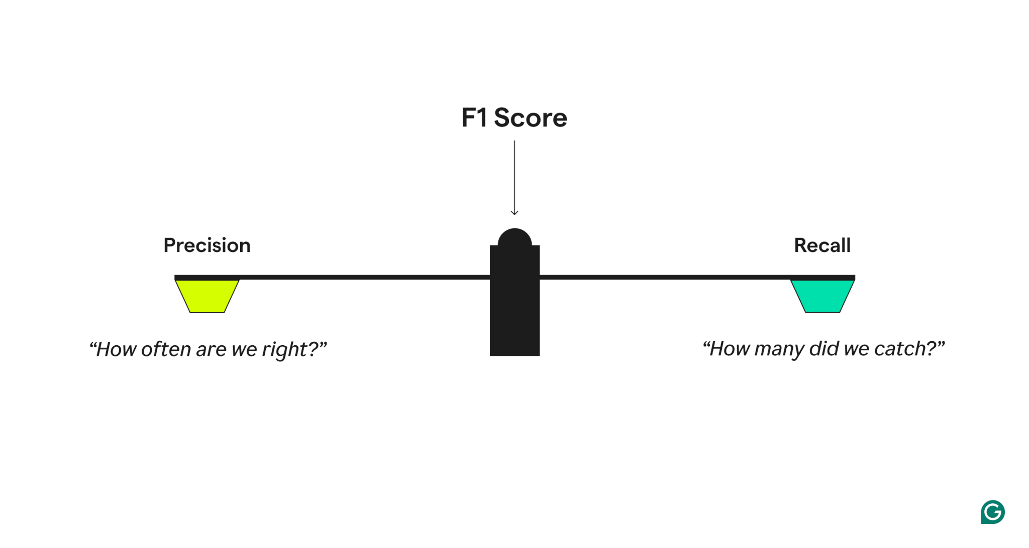
F1 Score as a Balance Between Precision and Recall — The F1-Score can be thought of as a balance between Precision ("How often are we right?") and Recall ("How many did we catch?"). It gives a good overall measure of a classifier's performance when both false positives and false negatives are important.

The formula for the F1-Score is:

F_{1} = 2 \cdot \frac{Precision \cdot Recall}{Precision + Recall}

Practical Implementation with Scikit-learn

Now, let's put theory into practice. Your background with Scikit-learn will be very helpful here. The sklearn.metrics module provides all the tools we need. The most convenient is classification_report, which computes all these metrics for you in one go.

Let's see how to generate and interpret this report.

Precision vs. Recall: Differences, Use Cases & Evaluation - V7 Go

The V7 Labs article also includes a practical section showing how to compute these metrics in Python.

Please read the section 'Tools to Compute Precision and Recall'. Focus on the Python code examples using precision_score, recall_score, and especially classification_report.

Code Walkthrough: Evaluating a Flaky Test Classifier

The following Python code simulates our flaky test scenario. It creates an imbalanced dataset, trains a RandomForestClassifier (as we did in a previous lesson), and evaluates it using classification_report.

import pandas as pd
from sklearn.datasets import make_classification
from sklearn.model_selection import train_test_split
from sklearn.ensemble import RandomForestClassifier
from sklearn.metrics import classification_report, accuracy_score




# 1. Create a synthetic imbalanced dataset
# 98% of data belongs to class 0 (stable), 2% to class 1 (flaky)
X, y = make_classification(
    n_samples=2000,
    n_features=20,
    n_informative=5,
    n_redundant=5,
    n_classes=2,
    weights=[0.98, 0.02], # This creates the imbalance
    flip_y=0.05,
    random_state=42
)

X_train, X_test, y_train, y_test = train_test_split(X, y, test_size=0.3, random_state=42, stratify=y)

print(f"Training set class distribution: {pd.Series(y_train).value_counts(normalize=True)}")
print(f"Test set class distribution: {pd.Series(y_test).value_counts(normalize=True)}\n")





# 2. Train a classifier
# Note: We are not using SMOTE here to better illustrate the evaluation on raw imbalanced data.
# In a real project, you would use the pipeline from the previous lesson.
clf = RandomForestClassifier(random_state=42, class_weight='balanced')
clf.fit(X_train, y_train)
y_pred = clf.predict(X_test)





# 3. Evaluate the model
# First, let's check the misleading accuracy
accuracy = accuracy_score(y_test, y_pred)
print(f"Overall Accuracy: {accuracy:.4f}\n")




# Now, let's get the metrics that matter
print("--- Classification Report ---")



# '1' is our positive class (flaky)
# '0' is our negative class (stable)
report = classification_report(y_test, y_pred, target_names=['Stable (0)', 'Flaky (1)'])
print(report)

Interpreting the Output

When you run this code, you'll get an output similar to the one shown in this image.

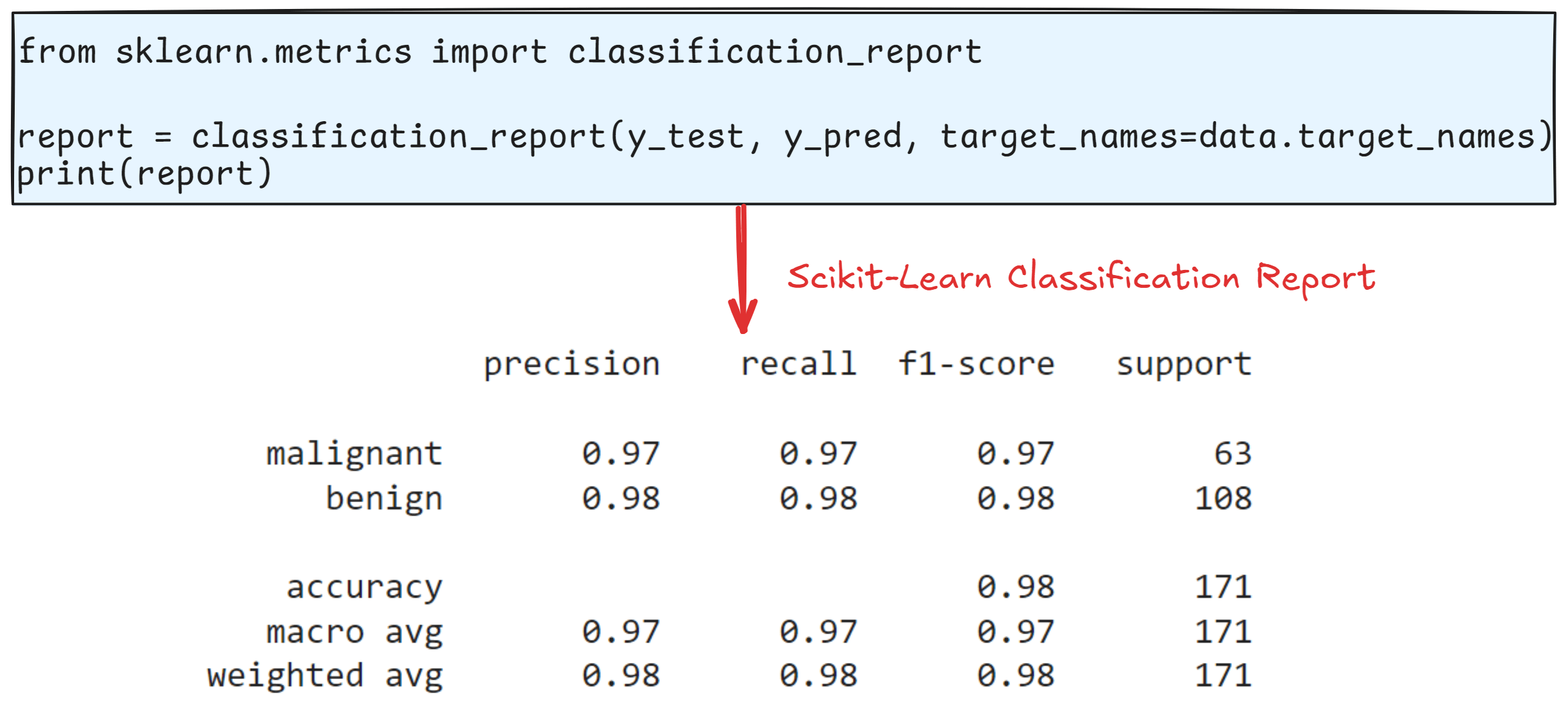
Scikit-Learn Classification Report Example — This is an example of a `classification_report` from Scikit-learn. It neatly summarizes the precision, recall, and f1-score for each class, along with support (the number of samples in each class). The macro and weighted averages provide an overall performance summary.

Let's break down the report from our code:

precision for Flaky (1): Of all tests we predicted as flaky, what percentage was correct?
recall for Flaky (1): Of all actual flaky tests, what percentage did we find?
f1-score for Flaky (1): The balanced score for our ability to detect flaky tests. This is often the most important number for the minority class.
support: Shows the number of actual instances of each class in the test set. This immediately confirms the class imbalance.
weighted avg: This is the average of each metric, weighted by the number of samples in each class (support). This is generally the most useful average score to report for an imbalanced dataset.

You'll notice the accuracy is very high, but the recall for the 'Flaky' class might be lower. This report gives you the detailed insight you need to understand your model's true strengths and weaknesses.

Conclusion

You have now learned how to properly evaluate a classification model, a skill that is absolutely essential for building production-ready ML tools for software quality.

Key Takeaways:

Accuracy is a misleading metric for imbalanced datasets, which are common in QA tasks like flaky test detection.
The Confusion Matrix (TP, TN, FP, FN) is the basis for more informative metrics.
Precision measures the cost of false positives (labeling a stable test as flaky). A high-precision model is trustworthy.
Recall measures the cost of false negatives (missing an actual flaky test). A high-recall model is thorough.
The F1-Score is the harmonic mean of precision and recall, providing a single, balanced metric to judge performance.
Scikit-learn's classification_report is the standard tool for generating these metrics in Python.

Preview of the Next Lesson:
In this lesson, we focused on evaluating classifiers. In the next lesson, we will do the same for the ranking model you built, diving into the NDCG metric we briefly touched upon. After that, we will tackle model interpretability, using tools like SHAP to answer the crucial question: why did the model make a specific prediction? This will complete your toolkit for building and assessing robust models.

Recommended resources