Saving and Loading Machine Learning Models

Introduction

Welcome back! In our last session, you successfully created a train.py script to train a bug-fix prediction model, evaluate it on imbalanced data, and use MLflow to systematically track your experiments. You logged the model as an MLflow artifact, which is excellent for reproducibility and comparison.

However, to "ship" our tool or integrate it into another application, we need a more direct and portable way to save our prediction logic. The learning outcome for this lesson is to persist the trained model and its associated artifacts (e.g., vectorizer, scaler). This means packaging all the necessary components—the preprocessing steps and the trained classifier—into a single, loadable file that can make predictions on new, raw data.

This lesson bridges the gap between the training environment and a production/inference environment, a critical step in building a real-world ML application.

Part 1: Anatomy of a Complete Prediction Pipeline

So far, we have treated preprocessing and model training as separate steps. We created a preprocessor.joblib file to transform data and a separate script to train the model on that transformed data.

For inference on new data, this separation is clumsy. An ideal workflow would take raw data as input and produce a prediction in one go. To achieve this, we need to bundle our fitted preprocessor and our trained model into a single, cohesive unit.

The scikit-learn library provides an elegant solution for this: the Pipeline object. A pipeline chains together multiple steps (e.g., transformers and an estimator) so that they can be treated as a single object.

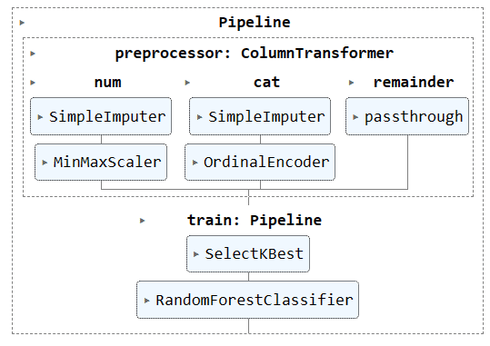
Scikit-learn Machine Learning Pipeline Structure — This diagram illustrates how a Scikit-learn Pipeline can combine a complex preprocessor (handling numerical and categorical data differently) with a final model (like a RandomForestClassifier). The entire assembly can be treated as a single estimator.

By wrapping our ColumnTransformer (the preprocessor) and our RandomForestClassifier in a Pipeline, we create a single object that encapsulates the entire prediction logic. When we call .fit() on this pipeline, it fits the preprocessor on the data, transforms it, and then trains the model on the transformed data. When we save this single fitted pipeline, we are persisting all the necessary artifacts at once.

Part 2: Choosing a Method to Persist Your Pipeline

Once we have our fitted pipeline object, how do we save it to a file? This process is called serialization—converting a Python object into a byte stream that can be stored on disk and later reconstructed.

There are several ways to do this in Python, each with its own trade-offs regarding security, efficiency, and compatibility.

Model persistence

The scikit-learn documentation provides excellent guidance on choosing the right method for saving your model. Let's walk through their decision process to understand our options.

First, read the decision guide that starts with the question 'Do you need the Python object after persistence...'. Next, review the section 'pickle, joblib, and cloudpickle' to see the basic code for saving and loading. Finally, read the critical 'Security & Maintainability Limitations' section. Focus on why joblib is often preferred for scikit-learn objects containing large NumPy arrays and be sure to understand the security risks and versioning challenges.

Key Takeaways from the Documentation:

pickle: The standard Python library for serialization. It works for almost any Python object.
joblib: Part of the SciPy ecosystem, joblib.dump and joblib.load are essentially wrappers around pickle but are more efficient for objects that contain large NumPy arrays, which is common in scikit-learn estimators. This makes it a preferred choice for our use case.
Security Risk: pickle and joblib are not secure. Loading a pickled file from an untrusted source can execute arbitrary malicious code. You should only load files that you have created or that come from a verified source.
Versioning: A model saved with one version of scikit-learn (e.g., 1.4.0) is not guaranteed to load correctly with another version (e.g., 1.5.0). It's crucial to pin your library versions (e.g., in a requirements.txt file) to ensure the environment is reproducible.

For our project, we will use joblib as it is the standard and most efficient method for persisting scikit-learn pipelines.

Part 3: Your Task: Create a `build_pipeline.py` Script

Now, let's create a script that assembles our full pipeline, trains it on the entire dataset, and saves the final, shippable artifact. This approach is superior to saving separate files because it creates a single, robust object that manages the entire workflow from raw data to prediction.

When moving to production, it's common practice to retrain your final model on all available data (both training and testing sets) to give it the most information to learn from. Our script will do just that.

Step 1: Create the `build_pipeline.py` Script

In your src/ directory, create a new file named build_pipeline.py. This script will load the raw data, load the fitted preprocessor we built in a previous lesson, combine it with a classifier into a final pipeline, and save it.

import pandas as pd
import joblib
import sys

from sklearn.ensemble import RandomForestClassifier
from sklearn.pipeline import Pipeline

if __name__ == "__main__":
    if len(sys.argv) != 4:
        print("Usage: python src/build_pipeline.py <raw_data_path> <preprocessor_path> <output_path>")
        sys.exit(1)

    raw_data_path = sys.argv[1]
    preprocessor_path = sys.argv[2]
    output_path = sys.argv[3]

    print("1. Loading raw data and fitted preprocessor...")



    # Load the raw commit data
    df = pd.read_csv(raw_data_path, parse_dates=['commit_date'])
    df = df.dropna(subset=['commit_message']) # Ensure no missing messages




    # Load the preprocessor that was fitted on the training data
    preprocessor = joblib.load(preprocessor_path)




    # Define the features (X) and target (y)
    X = df
    y = df['is_bugfix']

    print("2. Defining the final model pipeline...")



    # Define the final model. We can use the hyperparameters from our best MLflow run.
    model = RandomForestClassifier(
        n_estimators=100, 
        max_depth=10, 
        random_state=42,
        class_weight='balanced'
    )
    



    # Create the full pipeline by chaining the preprocessor and the model
    full_pipeline = Pipeline([
        ('preprocessor', preprocessor),
        ('classifier', model)
    ])

    print("3. Training the final pipeline on all data...")



    # Train the pipeline on the entire dataset
    full_pipeline.fit(X, y)

    print(f"4. Saving the final pipeline to {output_path}...")



    # Save the entire fitted pipeline object
    joblib.dump(full_pipeline, output_path)

    print("\nPipeline built and saved successfully!")

Step 2: Run the Script

Execute the script from your project's root directory. You'll need to provide paths to your raw commit data, the preprocessor you saved, and the desired output location for your final pipeline artifact.




# Make sure the output directory exists
mkdir -p artifacts




# Run the script
python src/build_pipeline.py data/raw/commits.csv artifacts/preprocessor.joblib artifacts/bugfix_pipeline.joblib

After running this, you will have a single file, bugfix_pipeline.joblib, inside an artifacts/ directory. This file contains everything needed to predict whether a new commit is a bug fix.

Part 4: Organizing for Deployment

This single artifact is the core of your shippable tool. In a typical production setup, this file would be stored alongside the application code that loads and uses it.

ML Model Deployment Project Structure — This image shows a common project structure for deploying a model. Our `bugfix_pipeline.joblib` would be analogous to the `model.pkl` file, stored and ready to be loaded by the application (`main.py`).

By creating a self-contained pipeline artifact, we've made the next step—building an inference service—much simpler. The service only needs to load this one file and pass new data to its .predict() method.

Conclusion

Excellent work! You have successfully packaged your entire machine learning workflow—from preprocessing to classification—into a single, persistent artifact. This is a major milestone in turning your model into a practical, reusable tool.

Key Takeaways:

To create a shippable ML tool, you must persist all fitted components, including preprocessors and the model.
scikit-learn's Pipeline object is the best practice for bundling transformers and an estimator into a single, cohesive unit.
joblib is the preferred method for serializing scikit-learn objects, but you must be aware of its security vulnerabilities and versioning dependencies.
The final artifact should be trained on all available data to maximize its performance.

Preview of the Next Lesson:
Now that we have our bugfix_pipeline.joblib artifact, what can we do with it? In the next lesson, you will implement a prediction function or class that encapsulates the full inference pipeline. We will write a script that loads our saved pipeline and uses it to make predictions on new, unseen commit data, completing the round trip from training to inference.

Recommended resources