Understanding Mixed-Effects Model Output

Welcome to our next lesson on advanced statistical modeling. In our previous session, you successfully fit your first random-intercept mixed-effects model using lme4::lmer(). This was a major step, moving from the why of mixed models to the practical how. You've seen the summary() output, and now it's time to decipher it.

This lesson focuses squarely on interpretation. Our goal is to equip you with the skills to read the output of a mixed model and translate its numbers into meaningful insights about your data. We will systematically break down the two main components of the summary: the fixed effects, which describe population-level trends, and the variance components (or random effects), which quantify the variability between your study subjects or groups. Mastering this is fundamental to your goal of conducting and reporting high-quality clinical research.

The Anatomy of an `lmer` Summary

Let's begin by recalling the structure of the model summary. As you saw in the last lesson, running summary() on a fitted lmer object produces an output with distinct sections.

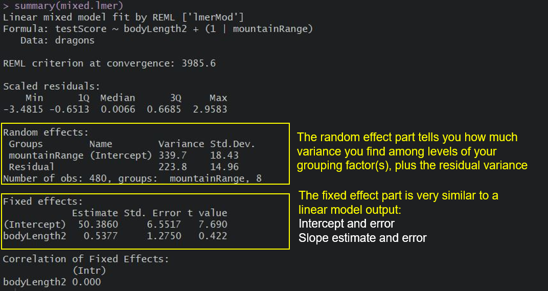
This annotated image of an `lmer` summary highlights the two key sections we'll be exploring: the **Random effects**, which describes the variance structure, and the **Fixed effects**, which contains the model's coefficients.

We will examine each of these sections in turn, starting with the one that should feel more familiar.

Interpreting Fixed Effects: The Population Average Story

The "Fixed effects" table in the lmer summary is your guide to the overall, population-level relationships in your data. The interpretation of these coefficients is very similar to how you would interpret coefficients from a standard linear model (lm()) or generalized linear model (glm()). They represent the average effect of a predictor on the outcome across all subjects or groups.

To make this concrete, let's return to the simulated pre-test/post-test Randomized Controlled Trial (RCT) example from the previous lesson, where we fitted the ANCOVA-style mixed model.

Just use multilevel models for your pre/post RCT data

This blog post by Solomon Kurz, which we used previously, provides the perfect context for understanding fixed effects.

First, quickly review the model formula under the heading "Multilevel models". Focus on the second formula, for the ANCOVA model, and the author's explanation of what each β coefficient represents. Next, scroll down to the R output for that model, labeled summary(l2). Examine the table under the "Fixed effects:" header. We will walk through this table together.

Let's break down the summary(l2) fixed effects table:

	Estimate	Std. Error	t value
(Intercept)	0.11320	0.09143	1.238
time	-0.12520	0.12549	-0.998
time:tx	1.17479	0.16286	7.213

(Intercept) (0.11320): In this model, this is the estimated mean value of the outcome y at baseline (time = 0) for all participants. The model assumes both control and treatment groups start from the same average point before the intervention.
time (-0.12520): This is the estimated change in the outcome y for the control group from baseline to the post-test measurement. Here, the outcome for the control group is expected to decrease by 0.125 units on average.
time:tx (1.17479): This is the interaction term and often the coefficient of primary interest in an RCT. It represents the additional change for the treatment group compared to the control group. To find the total effect for the treatment group, you add this to the time coefficient: -0.12520 + 1.17479 = 1.04959. So, while the control group's outcome decreased, the treatment group's outcome increased by about 1.05 units. This time:tx coefficient is the estimated average treatment effect.

The Std. Error gives you the uncertainty around each estimate, and the t value is the estimate divided by the standard error. As we noted before, lme4 deliberately omits p-values for these t-values due to complexities in calculating degrees of freedom. We will learn how to assess significance and report these results in a later lesson.

For a clear, conceptual walkthrough of interpreting fixed effects, the following video is excellent.

Interpreting fixed and random effects in mixed models

This video from the Simplistics (QuantPsych) channel provides an intuitive explanation using a different dataset.

Watch the segment explaining fixed effects interpretation. Notice how the presenter emphasizes that the interpretation is nearly identical to standard regression, but it represents the average effect across all the clusters (in this case, people).

Interpreting Variance Components: The Between- and Within-Group Story

Now we turn to the "Random effects" part of the summary, which is unique to mixed models. This section tells you how variability in your outcome is partitioned. In a random-intercept model, we are partitioning the total variance into two parts:

Between-group variance: How much do the groups (e.g., subjects) differ from each other in their baseline levels?
Within-group variance: How much do individual observations vary within the same group?

Let's look at the "Random effects" table from our summary(l2) example again:

Groups	Name	Variance	Std.Dev.
id	(Intercept)	0.3801	0.6165
Residual		0.4558	0.6752

id (Intercept): This line quantifies the between-subject variance. The Variance (often written as $σ_{u 0}^{2}$ ) is 0.3801. The Std.Dev. ( $σ_{u 0}$ ) is 0.6165. The standard deviation is often more interpretable: it suggests that a typical subject's personal intercept deviates from the overall fixed intercept (0.11320) by about ±0.62. This quantifies the extent of individual differences at baseline.
Residual: This line quantifies the within-subject variance (or residual variance, $σ_{ϵ}^{2}$ ). The Variance is 0.4558. The Std.Dev. ( $σ_{ϵ}$ ) is 0.6752. This tells you how much individual data points for a given subject scatter around that subject's own regression line.

The following plot visually represents what these random intercepts look like. The fixed intercept is the average starting point (the black line's intercept), while the random intercept variance quantifies how much the colored lines' starting points spread out around that average.

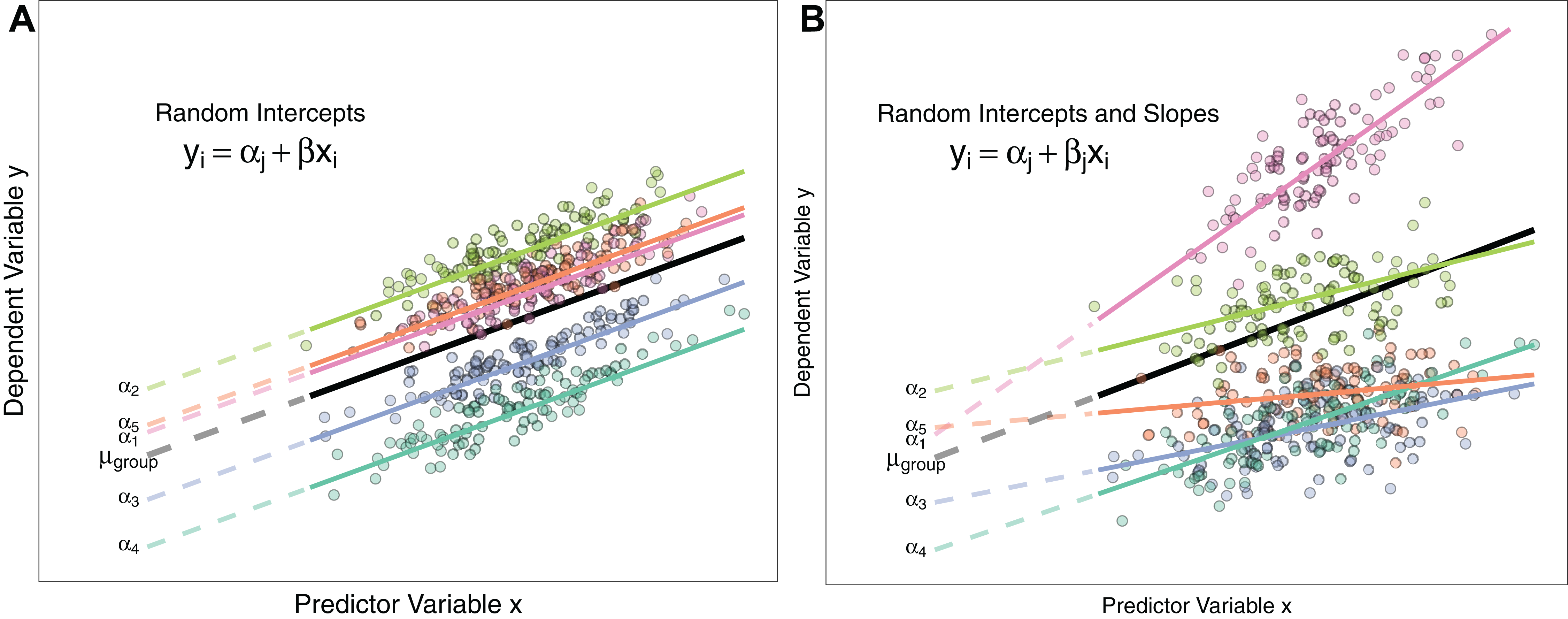
Panel A shows a random-intercepts model. The thick black line is the fixed effect (population average). The thinner colored lines represent individual groups. The random intercept variance quantifies the vertical spread of these lines' intercepts around the black line's intercept.

To solidify this concept, let's see it in action from first principles.

Simulate! Simulate! - Part 2: A linear mixed model

This blog post provides a brilliant demonstration by simulating data with known parameters and then fitting a model to see if it can recover them.

Read the first part of the post, up to the section "Make a function for the simulation". Pay close attention to how the author sets the parameters: mu = 10 (the fixed intercept), sds = 2 (the standard deviation for the random stand effect), and sd = 1 (the standard deviation for the residual effect). Then, look at the output from fit1. Notice how the estimated (Intercept) is close to 10, and how the Std.Dev. values for stand (Intercept) and Residual are close to the true values of 2 and 1. This makes the meaning of these numbers very tangible.

The Intraclass Correlation Coefficient (ICC)

From the variance components, we can calculate one of the most important descriptive statistics in a mixed model: the Intraclass Correlation Coefficient (ICC). The ICC tells you what proportion of the total variance in the outcome is due to systematic differences between the groups.

The formula is:

ICC = \frac{Variance _{between-groups}}{Variance _{between-groups} + Variance _{within-groups}} = \frac{σ _{intercept}^{2}}{σ _{intercept}^{2} + σ _{residual}^{2}}

Using the variances from our l2 model:

ICC = \frac{0.3801}{0.3801 + 0.4558} = \frac{0.3801}{0.8359} \approx 0.455

This means that about 45.5% of the total variance in the outcome y is attributable to differences between individuals. An ICC this high strongly confirms that the observations are not independent and provides a solid justification for using a mixed model instead of a simple linear model.

This video provides an excellent summary of interpreting both variance components and residuals.

Interpreting fixed and random effects in mixed models

Let's return to the Simplistics video for a final conceptual recap.

Watch the sections on interpreting random effects (the standard deviations), residual variance, and the final summary. The visual explanation of how intercepts and slopes vary is particularly helpful.

Reporting Model Results with `broom.mixed`

Finally, since your goal is to produce publication-quality analyses, it's crucial to know how to extract these results programmatically. Copy-pasting from the R console is inefficient and prone to error. The broom package family provides functions to turn model summaries into tidy data frames. For lmer objects, we use the broom.mixed package.

Simulate! Simulate! - Part 2: A linear mixed model

Let's see how broom.mixed simplifies our lives.

Read the section "Extract results". Notice how tidy(fit1) provides all the key parameters in a single, clean table. Pay special attention to the effects and scales arguments, which allow you to request only the fixed effects, only the random effects, and to get the random effects as variances (vcov) instead of the default standard deviations.

Using broom.mixed::tidy() is a key skill for reproducible reporting, allowing you to easily pass model results into tables using knitr::kable() or to create plots of coefficients.

Conclusion

In this lesson, you have learned to dissect and interpret the summary of a linear mixed-effects model. This moves you beyond simply running the code to truly understanding what the model is telling you about your data.

Key Takeaways:

Fixed Effects represent population-average relationships, and their coefficients are interpreted much like in standard regression.
Variance Components partition the total variance into between-group (e.g., (Intercept)) and within-group (Residual) sources.
The standard deviation of the random intercept quantifies the typical deviation of a group's intercept from the overall average.
The Intraclass Correlation Coefficient (ICC) is a critical metric derived from variance components that measures the degree of non-independence in your data. An ICC > 0 indicates that a mixed model is warranted.
The broom.mixed package is the standard tool for extracting model results into a tidy format for reporting.

Preview of the Next Lesson:

Now that you can fit a model and interpret its parameters, the next logical step is to use it to make predictions. In our next lesson, we will explore how to generate predictions from your lmer model for different predictor values and visualize these predictions along with their uncertainty.

Recommended resources

The Anatomy of an lmer Summary