Welcome to the next stage of your journey into advanced statistical modeling. In our last lesson, you learned to fit a random-intercept mixed model with lme4::lmer() and, crucially, how to interpret the fixed effects and variance components from its summary output. You now understand what the model's parameters represent.
This lesson builds directly on that foundation by answering the question: "Now that I have a fitted model, what can I do with it?" We will focus on one of the most powerful applications of a statistical model: making predictions. You will learn how to generate predictions from your lmer model, which is a fundamental skill for visualizing results, checking model fit, and communicating your findings—all essential steps in producing the high-quality research analyses you aim for.
Population vs. Subject-Specific Predictions
Before we write any code, it's vital to understand that a mixed-effects model can generate two different kinds of predictions. The distinction between them is at the very heart of why we use these models.
-
Population-Level (or Marginal) Predictions: These predictions are based only on the model's fixed effects. They represent the predicted outcome for an "average" subject or group, ignoring the specific random effect associated with any single individual. This is useful for describing the overall trend in the population.
-
Subject-Specific (or Conditional) Predictions: These predictions use both the fixed effects and the estimated random effects. They represent the predicted outcome for a particular subject or group in your dataset, taking into account their unique deviation from the population average.
This image provides a great visual for this concept.
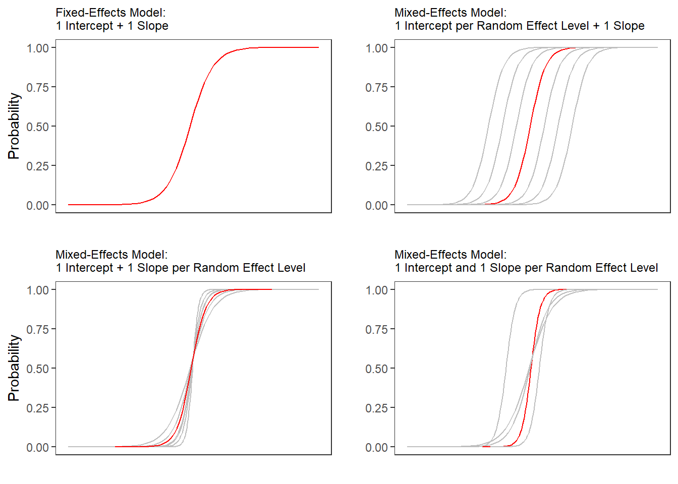
Our goal in this lesson is to learn how to generate the data for both the red line and the grey lines using R.
Generating Subject-Specific Predictions with predict() and augment()
Let's start by generating predictions for the specific individuals that are already in our dataset. The simplest tool for this is R's built-in predict() function.
Chapter 9 Linear mixed-effects models | An R companion to Statistics
This resource from "An R companion to Statistics" provides a concise example of using predict().
Please read the section "Plotting model predictions". Notice how a new column, pred, is created by calling predict(modg) and is then used in a ggplot call to visualize the subject-specific lines.
As you saw, predict() is straightforward. However, in a modern tidyverse workflow, it's often more convenient to use the augment() function from the broom package. You've already seen broom.mixed::tidy() for summarizing model parameters; augment() is for adding model outputs (like predictions) to your original data.
When you use augment() on an lmer object, it adds several columns to your data frame, the most important of which is .fitted. This column contains the subject-specific predictions.
Let's see a practical example of visualizing these individual predictions.
Chapter 20 Linear mixed effects models 4 | Psych 252
This chapter from "Psych 252" has excellent, clear code examples for plotting predictions.
Read the subsection "Data with individual model predictions". The code first uses augment() to create a new data frame df.plot which includes the original data plus the model's outputs. Then, examine the ggplot code that follows. The key part is geom_line(mapping = aes(y = .fitted), color = "red"). This line is what draws the prediction lines for each participant, using the values from the .fitted column that augment() created. The result is a plot showing the model's prediction for every single participant in the study.
Using augment() is a powerful way to see what the model has "learned" about each of your subjects. By plotting the .fitted values against the raw value, you can visually assess how well the model is capturing the individual trajectories.
Generating Population-Level Predictions with ggeffects
While individual predictions are useful, for publications and presentations, we often want to show the overall, population-level trends. We want to plot the "red line" from the diagram at the beginning of the lesson.
For this task, the ggeffects package is exceptionally useful. Its main function, ggpredict(), calculates predicted values for specified terms in your model, holding other predictors at their mean or reference level. Crucially, it calculates these predictions based only on the fixed effects, giving us the population-level estimates we want. It also calculates the corresponding confidence intervals, which are essential for quality visualizations.
Chapter 20 Linear mixed effects models 4 | Psych 252
Let's return to the "Psych 252" chapter for another excellent example.
Read the subsection "Data with overall model predictions". First, look at the call to ggpredict(). df.model = ggpredict(model = fit, terms = c("timepoint", "condition"), type = "fixed") Here, we ask for predictions across the timepoint and condition variables. The key argument is type = "fixed", which tells ggpredict to compute population-level predictions. The function returns a new data frame, df.model, containing columns for the predicted values (predicted), and the lower and upper bounds of the confidence interval (conf.low, conf.high). Next, look at the ggplot code. It plots the raw data (faintly in the background) and then overlays the results from ggpredict. The confidence interval is plotted using geom_ribbon(...), and the mean prediction is plotted with geom_line(...). This is a classic and highly effective way to visualize model results.
The combination of ggpredict() to generate a tidy data frame of predictions and ggplot2 to plot them is a workflow you will use constantly in your research. It provides a direct path from a fitted model to a publication-quality figure that clearly communicates the key findings.
A Note on Predictions for New Data
So far, we have generated predictions for the data we used to fit the model. You can also generate predictions for new, hypothetical data points. Both predict() and ggpredict() can accept a newdata argument, which should be a data frame with columns matching the predictor names in your model.
For mixed models, there's a nuance:
- To get population-level predictions for new data, you can use
ggpredict()as you've just seen, or you can usepredict()with the argumentre.form = ~0, which tells it to ignore the random effects. - To get subject-specific predictions for a new data point, you must specify which subject the new data belongs to by including their ID in the
newdatadata frame.
We won't dive deeper into newdata now, but it's good to know this capability exists for when you need to predict outcomes for a new patient or scenario not in your original dataset.
Conclusion
In this lesson, you've learned how to take a fitted lmer model and use it to make predictions. This is a critical bridge between fitting a model and communicating its story.
Key Takeaways:
- Mixed models can produce two types of predictions: subject-specific (conditional on random effects) and population-level (based on fixed effects only).
- The
broom::augment()function is a tidy way to add subject-specific predictions (in the.fittedcolumn) to your original data frame for model checking and visualization. - The
ggeffects::ggpredict()function is a powerful tool for generating population-level predictions and their confidence intervals, creating the perfect input for creating summary plots. - Visualizing predictions is the best way to understand what they mean. The
ggplot2code you've seen today serves to make the generated prediction data tangible.
Preview of the Next Lesson:
You now know how to generate the data frames that contain model predictions. In our next lesson, we will focus entirely on the art of visualizing this data. We will take a deep dive into ggplot2, exploring how to customize plots of your model predictions to create sophisticated, clear, and publication-ready figures that effectively communicate your research findings.