Visualizing Predictions and Uncertainty

The Goal: Visualizing Layers of Information

A good visualization of a mixed-effects model often conveys multiple layers of information at once. We want to show the overall trend (the fixed effect) while also giving a sense of the underlying individual variation (the random effects).

Consider these two plots, which both visualize data from the sleepstudy dataset you may have encountered. This dataset tracks the reaction times of subjects over successive days of sleep deprivation.

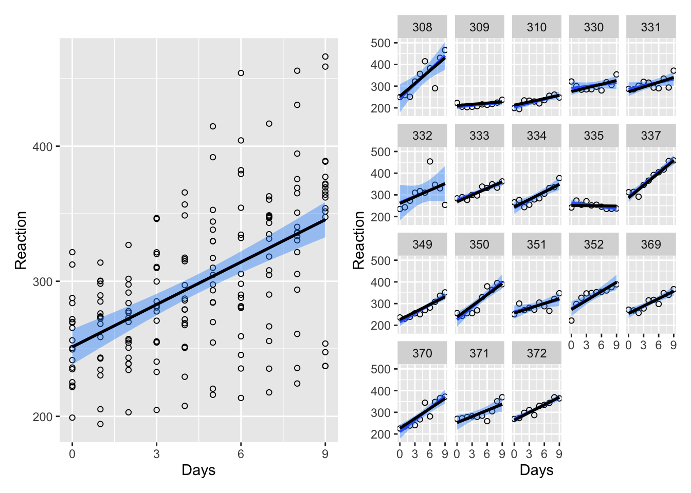
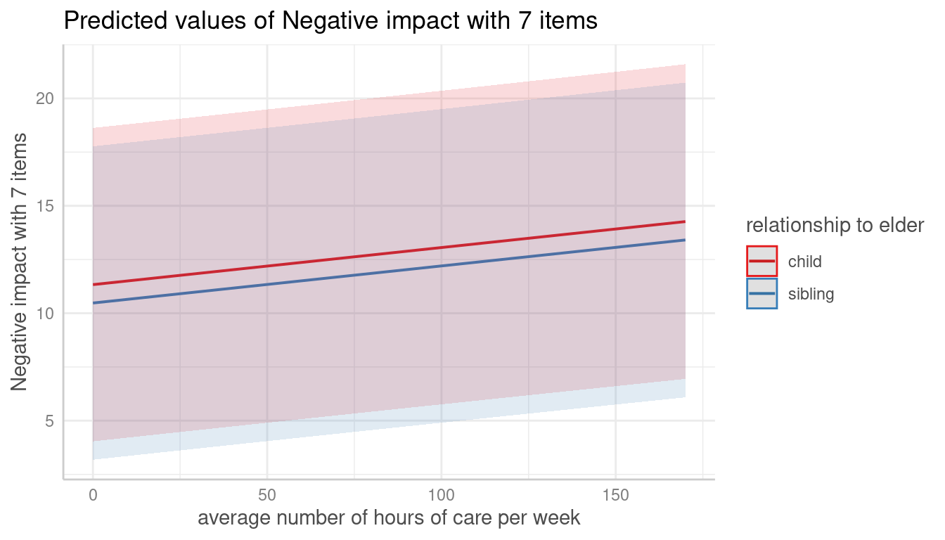
These plots effectively communicate the model's findings. Throughout this lesson, you will learn the techniques required to produce visualizations just like these.

The Core Workflow: ggeffects with ggplot2

In the last lesson, you used ggeffects::ggpredict() to generate a tidy data frame of population-level predictions, complete with confidence intervals (conf.low and conf.high). This data frame is designed to be used directly with ggplot2. The ggeffects package even provides a convenient plot() method that acts as a great starting point.

The workflow you just read about is incredibly powerful. By starting with the basic plot from ggeffects and adding ggplot2 layers, you have full control over the final appearance, allowing you to tailor it to the standards of any academic journal.

Let's imagine you've fit a model to the sleepstudy data:
fit <- lmer(Reaction ~ Days + (Days | Subject), data = sleepstudy)

You could generate population-level predictions and plot them like this:

# 1. Generate predictions
pred_pop <- ggpredict(fit, terms = "Days")




# 2. Create the plot
ggplot(pred_pop, aes(x = x, y = predicted)) +
  geom_line(linewidth = 1) +  # The main prediction line
  geom_ribbon(aes(ymin = conf.low, ymax = conf.high), alpha = 0.2) + # The confidence band
  labs(
    title = "Average Effect of Sleep Deprivation on Reaction Time",
    x = "Days of Deprivation",
    y = "Reaction Time (ms)"
  ) +
  theme_minimal()

This code would produce a plot similar to the left panel of the first image, showing the single, population-level trend with its associated uncertainty.

Telling the Whole Story: Combining Population and Individual Views

To truly represent a mixed model, you should also visualize the individual-level effects. A very effective technique is to plot the main population trend prominently, and then overlay the individual data or predictions more subtly in the background.

There are several ways to do this. A common approach is to add a geom_line layer that plots the reaction time for each subject.

# Continuing from the previous plot
ggplot(pred_pop, aes(x = x, y = predicted)) +
  geom_line(
    data = sleepstudy, # Switch to the original data for this layer
    aes(x = Days, y = Reaction, group = Subject), # Map aesthetics for individuals
    color = "grey", alpha = 0.5
  ) +
  geom_line(linewidth = 1.2, color = "blue") + # Re-plot the main line on top
  geom_ribbon(aes(ymin = conf.low, ymax = conf.high), alpha = 0.2, fill = "blue") +
  labs(
    title = "Effect of Sleep Deprivation on Reaction Time",
    subtitle = "Population average (blue) with individual trajectories (grey)",
    x = "Days of Deprivation",
    y = "Reaction Time (ms)"
  ) +
  theme_minimal()

Notice the key addition: geom_line(data = sleepstudy, aes(..., group = Subject), ...)
By specifying group = Subject, you are telling ggplot2 to draw a separate line for each subject, connecting their own data points across the days. This one addition adds a rich layer of context, showing both the overall trend and the variability between individuals that motivated using a mixed model in the first place.

The Express Lane: Quick and Powerful Plots with sjPlot

While building plots with ggplot2 gives you ultimate control, sometimes you need to quickly explore your model's predictions. This is where the sjPlot package shines. Its primary function, plot_model(), is a versatile tool that can visualize results from a huge variety of models, including lmer objects.

sjPlot is brilliant because it understands the model object and automatically generates the most appropriate visualization, often with just a single line of code.

For our sleepstudy model, visualizing the predictions would be as simple as:
plot_model(fit, type = "pred", terms = "Days")

For models with interactions or categorical predictors, plot_model() is particularly valuable, as it will intelligently create plots showing the predicted lines for each group, which is a common need in clinical research analysis. It's an indispensable tool for initial data exploration and for generating standard figures efficiently.

A Deeper Look at Uncertainty

All the plots we've discussed include a shaded region representing the confidence interval. But what does that band actually represent, and where does it come from?

The shaded band illustrates our uncertainty about the fixed effect. It's a plausible range for the true population average line. If we could repeat our study 100 times, we would expect the confidence interval from 95 of those studies to contain the true average line.

For complex models like lmer, these intervals can be difficult to calculate analytically. A common and robust method used under the hood is bootstrapping.

You don't need to implement bootstrapping by hand every time—packages like ggeffects and sjPlot handle it for you. But understanding that the confidence band represents the distribution of plausible results from resampling your data gives you a much deeper appreciation for the uncertainty inherent in your model.

Conclusion

You are now equipped with a powerful toolkit for visualizing the results of your advanced statistical models. This is a critical skill for interpreting your findings and communicating them to others.

Key Takeaways:

• The ggeffects + ggplot2 workflow provides a flexible and powerful way to create customized, publication-quality visualizations of model predictions.
• A key technique for mixed models is to plot the population-level trend prominently (e.g., a thick, colored line with a ribbon) and overlay individual trajectories more subtly (e.g., thin, grey lines).
• The sjPlot::plot_model() function is an invaluable tool for rapid exploration, capable of generating insightful plots from complex models with a single line of code.
• The shaded confidence band on a prediction plot visually represents our uncertainty about the true population average, often derived from methods like bootstrapping that simulate repeated experiments.

Preview of the Next Lesson:

Visualizations tell a powerful story, but scientific reports also require numerical summaries. In our next and final lesson of this module, you will learn how to extract the key results of your lmer model—such as fixed-effect coefficients, variance components, and their confidence intervals—into clean, tidy data frames using the broom.mixed package, preparing them for inclusion in tables and reports.