Tidying `lmer` Model Results with `broom.mixed`

The Problem: Model Objects are Messy

After you fit a model in R, for instance with lmer(), you get a model object. You've used summary() to print a useful overview of this object to the console. While this summary is great for a quick look, it's surprisingly difficult to work with programmatically. If you wanted to extract the p-value for a specific coefficient to put in a table, or plot the confidence intervals for all coefficients, you would need to write cumbersome and fragile code to parse the text output or navigate a deeply nested list structure.

This is a common frustration in R. Model objects are often complex and don't follow the "tidy data" principles that make packages like dplyr and ggplot2 so powerful.

As you saw, getting information out of a standard model summary involves multiple steps, dealing with information hidden in row names, and manually calculating values that are printed but not stored. This is inefficient and error-prone, especially when you need to report results from multiple models.

The Tidy Solution: The broom Package

The broom package was created to solve this exact problem. It provides a set of functions that convert the messy output of various statistical models into tidy data frames. A "tidy" data frame has a consistent structure: one observation per row, one variable per column.

The broom philosophy revolves around three main verbs, each for a different level of model summary:

1. tidy(): This function summarizes the components of the model. For a regression model, this typically means one row for each coefficient (or term) in the model, with columns for the estimate, standard error, p-value, etc.
2. augment(): This adds observation-level information to the original data used to fit the model. For example, it can add columns for fitted values (predictions) and residuals for each data point. You have already seen this in action, as packages like ggeffects use this principle to generate prediction data frames.
3. glance(): This provides a single-row summary of the entire model, containing statistics like R-squared, AIC, BIC, and the log-likelihood.

Tidying Mixed-Models with broom.mixed

The lmer models you've been working with are more complex than standard linear models. They have both fixed effects (the population-level coefficients like time_point) and random effects (the variance components, like the variance between subjects).

Because of this added complexity, the original broom package has been extended by broom.mixed, a package specifically designed to handle the output of mixed-effects models from lme4 and other similar packages.

Let's see it in action. First, make sure you have the package installed and loaded, along with lme4.

# install.packages("broom.mixed")
library(lme4)
library(broom.mixed)

Now, let's refit the sleepstudy model we've used before.

data(sleepstudy, package = "lme4")
fit <- lmer(Reaction ~ Days + (Days | Subject), data = sleepstudy)

First, let's look at the standard summary() output, which you've seen before. It's informative but not "tidy."

summary(fit)

## Linear mixed model fit by REML ['lmerMod']
## Formula: Reaction ~ Days + (Days | Subject)
##    Data: sleepstudy
## 
## REML criterion at convergence: 1743.6
## 
## Scaled residuals: 
##     Min      1Q  Median      3Q     Max 
## -3.9536 -0.4634  0.0231  0.4634  5.1793 
## 
## Random effects:
##  Groups   Name        Variance Std.Dev. Corr
##  Subject  (Intercept) 612.10   24.741       
##           Days         35.07    5.922   0.07
##  Residual             654.94   25.592       
## Number of obs: 180, groups:  Subject, 18
## 
## Fixed effects:
##             Estimate Std. Error t value
## (Intercept)  251.405      6.825  36.838
## Days          10.467      1.546   6.771
## 
## Correlation of Fixed Effects:
##      (Intr)
## Days -0.138

Now, let's apply broom.mixed::tidy() to the same fit object.

tidy(fit)

## # A tibble: 5 × 7
##   effect   group    term            estimate std.error statistic
##   <chr>    <chr>    <chr>              <dbl>     <dbl>     <dbl>
## 1 fixed    NA       (Intercept)       251.       6.82      36.8 
## 2 fixed    NA       Days               10.5      1.55       6.77
## 3 ran_pars Subject  sd__(Intercept)    24.7     NA         NA   
## 4 ran_pars Subject  cor__(Intercept)    0.0678  NA         NA   
## 5 ran_pars Residual sd__Observation    25.6     NA         NA

Look at that beautiful, clean data frame! This is a format you can immediately use with dplyr to filter, ggplot2 to plot, or feed into a table-making function.

Let's break down the columns:

• effect: Crucially, this tells you if the row refers to a fixed effect or a random-effect parameter (ran_pars).
• group: For random effects, this specifies the grouping factor (e.g., Subject).
• term: The name of the parameter. For fixed effects, these are your predictors. For random effects, they are standard deviations (sd__...) or correlations (cor__...).
• estimate: The calculated value for that term.
• std.error and statistic: The standard error and t-statistic for the fixed effects. These are NA for the default variance components because their statistical inference is more complex.

You can also ask tidy() to compute confidence intervals, which is very useful for reporting.

tidy(fit, conf.int = TRUE)

## # A tibble: 5 × 9
##   effect   group    term            estimate std.error statistic conf.low conf.high
##   <chr>    <chr>    <chr>              <dbl>     <dbl>     <dbl>    <dbl>     <dbl>
## 1 fixed    NA       (Intercept)       251.       6.82      36.8    238.      265.  
## 2 fixed    NA       Days               10.5      1.55       6.77     7.42      13.5 
## 3 ran_pars Subject  sd__(Intercept)    24.7     NA         NA       14.4       37.7 
## 4 ran_pars Subject  cor__(Intercept)    0.0678  NA         NA       -0.491      0.622
## 5 ran_pars Residual sd__Observation    25.6     NA         NA       22.9       28.9

This adds conf.low and conf.high columns, giving you the 95% confidence intervals for every parameter in your model, ready for reporting.

Application: Creating Publication-Quality Tables

The primary use of broom.mixed::tidy() is as a backend for other packages that create beautiful summary tables. Packages like modelsummary, gtsummary, and sjPlot are designed to take a model object and produce a publication-ready table. Under the hood, they use broom.mixed to extract the necessary information in a tidy format before arranging it into a table.

By using broom.mixed, these packages can generate beautifully formatted tables that clearly separate fixed and random effects, include confidence intervals and p-values, and can even place multiple models side-by-side for comparison.

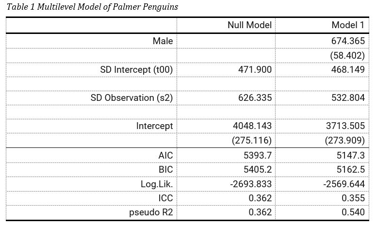
An example of a publication-quality table created with the modelsummary package, which relies on broom and broom.mixed to extract model results into a structured format.

Another example showing tidied model outputs from three different tests. This clean, consistent format is the direct result of using a tidying function like broom.mixed::tidy().

Beyond a Single Model

The true power of the tidy workflow becomes apparent when you work with many models. Imagine you have run a separate model for each gene in a genomic study, or for each country in a global health dataset. Because tidy() returns a data frame, you can run it on every model, and then stack the results into one large data frame for analysis and visualization. This is a workflow that combines purrr::map() with broom::tidy(), a pattern you may have seen before.

This ability to programmatically extract, combine, and analyze results from dozens or even thousands of models is central to modern, reproducible research and directly aligns with your goal of building an "extravagant" and industry-ready skill set.

Conclusion

In this lesson, you have learned one of the most important "glue" skills in the R data analysis ecosystem. You now understand the problem of messy model objects and how the broom and broom.mixed packages provide an elegant solution. By converting model outputs to tidy data frames, you unlock the ability to seamlessly integrate your statistical modeling results with the powerful tidyverse tools for manipulation, visualization, and reporting.

Key Takeaways:

• Standard R model objects are "messy," making it difficult to programmatically extract results.
• The broom package solves this by converting model objects into tidy data frames.
• The broom.mixed package extends this capability to handle complex mixed-effects models from lme4.
• The tidy() function is your primary tool for extracting model components (coefficients, variance components) into a clean, multi-row data frame.
• The output of tidy() is the essential ingredient used by packages like modelsummary and gtsummary to create publication-quality tables.
• Combining tidy() with functional programming tools like purrr::map() enables powerful, scalable analysis of multiple models.

Preview of the Next Lesson:

You have now completed the entire modeling workflow, from data import and transformation to advanced modeling and reporting. In our final module, we will zoom out to focus on the entire project. In the next lesson, you will learn how to structure your analyses for maximum reproducibility and ease of collaboration using the workflowr package, ensuring that your work is not only correct but also transparent and shareable.