Fitting Random-Intercept Models with `lmer()`

The lme4 Package and Data Format

The standard for fitting linear mixed-effects models in R is the lme4 package. If you don't have it installed, you can do so now by running install.packages("lme4") in your console. Once installed, we load it as usual with library(lme4).

Before we can model, we must address a critical data formatting requirement. lme4 and other mixed-modeling functions expect data to be in long format. This means each row represents a single observation for a single subject at a single time point.

This is often different from how clinical data is initially recorded. You might receive a dataset in wide format, where each row is a unique subject, and repeated measurements are in separate columns (e.g., weight_month1, weight_month2, weight_month3).

Let's look at a practical example of this transformation. A blog post by Solomon Kurz provides a clear demonstration using a simulated pre-test/post-test randomized controlled trial (RCT) dataset, a scenario you will encounter frequently.

The key takeaway is that for a mixed model, you need a column that identifies the grouping or clustering factor (in this case, id for the participant) and another column that identifies the repeated measure (e.g., time or visit_number).

The lmer() Formula Syntax

With our data in the correct long format, we can now build our model using the lmer() function. The formula syntax is an extension of what you already know from lm() and glm(), with a special component for specifying random effects.

The general structure is:
lmer(outcome ~ fixed_effects + (random_effects | grouping_variable), data = your_data)

Let's break this down:

• outcome ~ fixed_effects: This part is identical to a standard lm() formula. You list your dependent variable and the predictors whose population-average effects you want to estimate.
• (random_effects | grouping_variable): This is the new part. It tells lmer() what effects you want to allow to vary across the levels of your grouping_variable.
• grouping_variable: This must be a factor variable in your data that identifies the clusters (e.g., subject_id, hospital_id, classroom_id).

For today's lesson, we are focusing on the random-intercept model. In this model, we assume the relationship between the predictors and the outcome (the slope) is the same for all subjects, but the baseline level (the intercept) can vary from subject to subject.

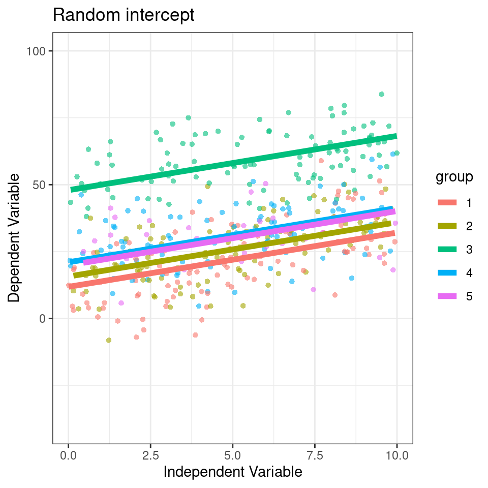
To specify a random-intercept model, the syntax is (1 | grouping_variable). The 1 is a placeholder for the intercept. So, a full random-intercept model formula looks like this:

lmer(outcome ~ predictor1 + predictor2 + (1 | subject_id), data = your_data)

The following resource provides a formal summary of the formula notation.

For a more conversational walkthrough of the syntax, this video provides an excellent summary.

Fitting a Random-Intercept Model in R

Let's now apply this knowledge to fit a model using the simulated RCT data from the Solomon Kurz article. In that example, researchers are interested in the effect of a treatment (tx) over time (time) on an outcome y. Because each participant (id) was measured twice (pre- and post-treatment), the observations are not independent, and a mixed model is appropriate.

The model is designed to estimate the treatment effect, which is captured by the interaction between time and tx.

Let's write and run this code ourselves. Assuming you have the long-format data frame dl from the first reading:

# Load the lme4 package
library(lme4)




# Fit the random-intercept model
# y is the outcome
# time and the interaction tx:time are fixed effects
# (1 | id) specifies a random intercept for each participant
model_fit <- lmer(y ~ 1 + time + tx:time + (1 | id), data = dl) 

That's it! You have successfully fit a random-intercept linear mixed-effects model. The model_fit object now contains all the results.

A First Look at the Model Summary

To see the results, we use the summary() function, just as with lm() and glm().

summary(model_fit)

The output can seem intimidating at first, but it is organized into logical sections.

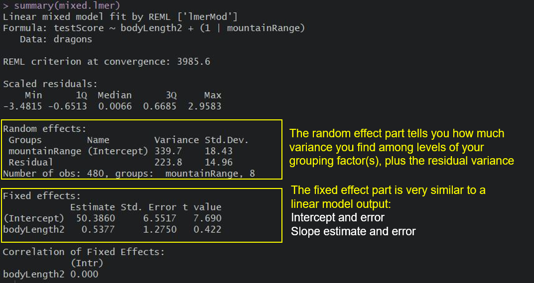
Let's break down what you're seeing:

1. Random effects: This section provides information about the variance components. In our random-intercept model, you'll see a variance estimate for your grouping factor (id (Intercept)) and for the Residual. The id variance tells you how much the intercepts vary from person to person. The Residual variance tells you how much variability remains for observations within the same person. We will dive deep into interpreting these variances in the next lesson.
2. Fixed effects: This section should look very familiar. It's almost identical to the coefficients table from an lm() summary. It shows the Estimate (the coefficient), Std. Error, and t value for each fixed predictor in your model (Intercept, time, and tx:time). These are your population-average effects.

One thing you'll notice is the absence of p-values in the fixed effects table. This is a deliberate choice by the lme4 authors due to the complexity of calculating degrees of freedom in mixed models. We will discuss how to assess the significance of fixed effects later. For now, focus on understanding the structure of the output.

Conclusion

In this lesson, you made the leap from the theory of mixed models to their practical application. You've learned the essential workflow for fitting a random-intercept model, which is a powerful and common tool for analyzing data from clinical studies.

Key Takeaways:

• The lme4 package is the primary tool for fitting linear mixed-effects models in R.
• lme4 requires data to be in long format, with one row per observation and a column identifying the grouping variable.
• The lmer() function uses an extended formula syntax: outcome ~ fixed_effects + (random_effects | group).
• A random-intercept model is specified with (1 | group), which allows the baseline for each group to vary while keeping the slopes constant.
• The summary() output is split into Random effects (showing between-group variance) and Fixed effects (showing population-average coefficients).

Preview of the Next Lesson:

Now that you can fit a model and identify the main sections of its output, our next step is to learn how to interpret these results in detail. We will dissect the summary() output, explaining how to interpret the fixed-effect coefficients in the context of your research question and how to understand and report the random-effect variance components.