Introduction
In the last lesson, you mastered ggsave(), giving you the ability to export a finished ggplot2 visualization as a high-quality, standalone file. This is a vital skill for preparing figures for submission. However, in research and data analysis, a plot rarely stands alone. It needs context: an introduction, a description of the methods, a summary of the results, and a conclusion. Your goal of producing analysis for academic theses and publications requires weaving together narrative, code, and visual output into a single, coherent story.
This lesson introduces you to the tool that makes this possible: R Markdown. You'll learn how to create documents that combine your written analysis with live R code, tables, and plots. Specifically, we will focus on the fundamental anatomy of an R Markdown file, breaking it down into its three core components: the YAML header, narrative text, and R code chunks. Understanding this structure is the first step toward creating fully reproducible reports, a cornerstone of modern data analysis.
1. From Script to Report: The Power of R Markdown
So far, you've been writing code in R scripts (.R files). These are excellent for organizing and running your code, but they are not designed for communication. An R Markdown file (.Rmd) is different. It's a plain-text document that allows you to blend formatted text with chunks of executable R code.
The magic happens when you "knit" an R Markdown document. This process, facilitated by the knitr and rmarkdown packages, runs all your R code and combines the output (like plots and tables) with your text to produce a polished, final document. This could be an HTML file for a website, a PDF for a paper, or a Word document for a collaborator.
This workflow is incredibly powerful because if your data changes, you don't need to manually copy and paste new plots or results. You simply knit the document again, and everything is updated automatically. This ensures your final report is always in sync with your analysis.
The image below illustrates this translation process. On the left is the R Markdown script, containing a mix of settings, text, and code. On the right is the resulting Word document, showing how each element has been rendered into a clean, professional report.
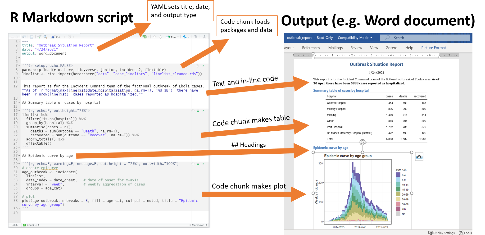
An R Markdown script combines metadata (YAML), narrative text, and R code chunks. When "knitted," it produces a formatted output document, such as this Word file, with all code results embedded.
2. Creating Your First R Markdown Document
Let's get started by creating your first .Rmd file. The process is straightforward in RStudio. The short video below demonstrates how to open a new R Markdown file and shows the default template RStudio provides.
This short video by Roger Peng provides a clear walkthrough of creating a new R Markdown file in RStudio.
Watch the clip from the beginning to see the process. Notice the pop-up window where you can set the title, author, and default output format. For now, leave the default as HTML.
When you create a new R Markdown file, RStudio populates it with a helpful template. Don't worry about understanding every line just yet. For now, simply observe the different kinds of content in the file. You'll see some text at the top between --- lines, some regular text with ## symbols, and some gray boxes containing R code. These are the three fundamental components we're about to explore.
3. The Anatomy of an R Markdown File
Every R Markdown document is composed of three basic parts. Understanding the role of each is key to using R Markdown effectively.
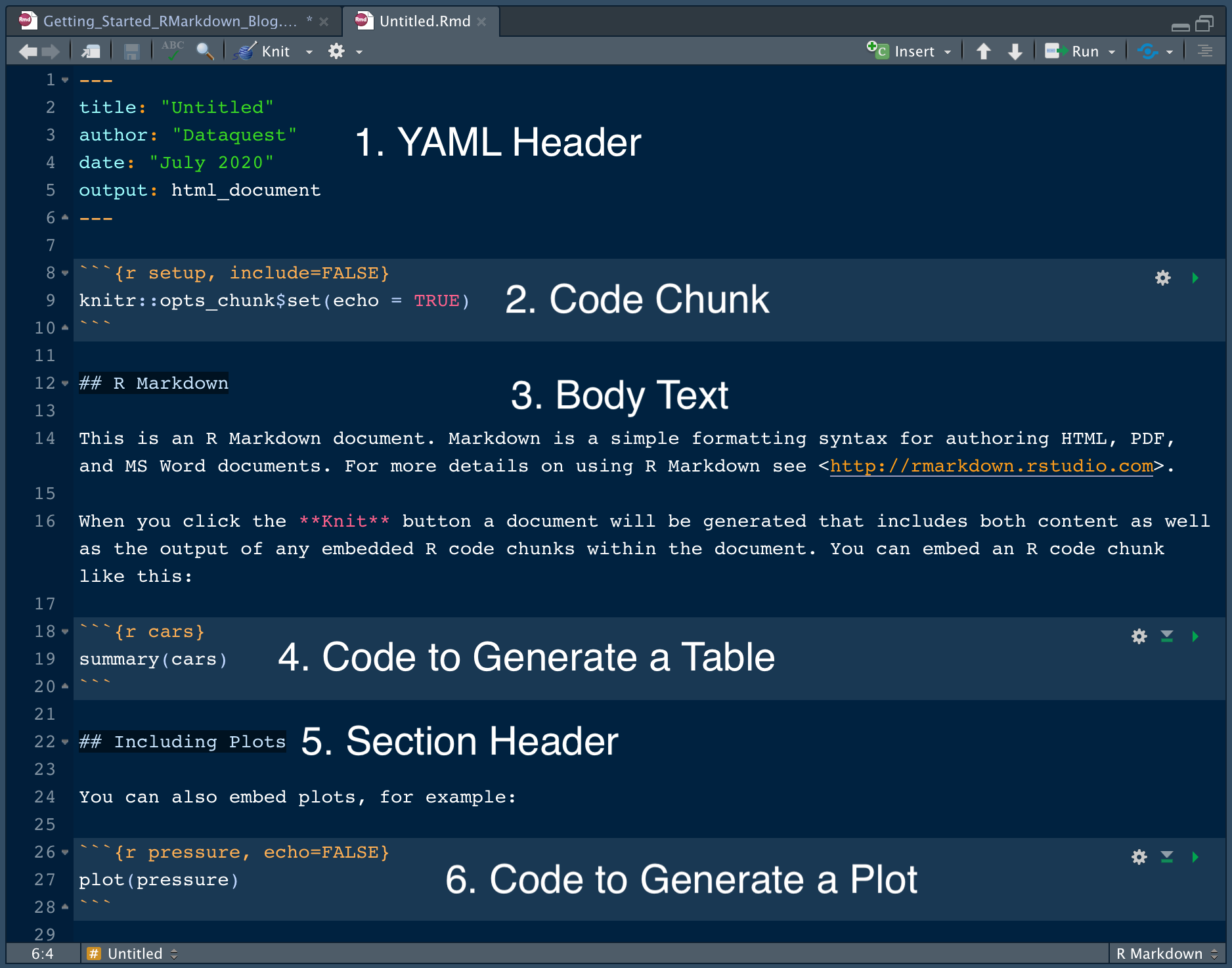
The three main components of an R Markdown file are the YAML Header (1), the Body Text (3, 5), and Code Chunks (2, 4, 6).
Let's break these down one by one, using the image above as our guide.
a) The YAML Header
At the very top of the document, enclosed by a pair of --- lines, is the YAML header. YAML stands for "YAML Ain't Markup Language," and it's a simple, human-readable format for storing configuration data.
In R Markdown, the YAML header acts as the document's control panel. It holds metadata such as the title, author, and date. Most importantly, it specifies the output format.
27 R Markdown - R for Data Science - Hadley Wickham
The "R for Data Science" book provides a concise definition of the components.
Read the first point in the list, which formally introduces the YAML header.
The output setting is particularly powerful. By changing just one line in the YAML header, you can completely alter the type of file you produce. The following video demonstrates this by changing the output from the default html_document to word_document and even a PowerPoint presentation.
Introduction to R Markdown | Foundations of data analysis with R (lesson 6)
This video from The GRAPH Courses clearly demonstrates the function of the YAML header.
Watch the segment from where the presenter explains the YAML header and modifies the output: field to create a Word document. You can stop before the discussion on PowerPoint.
b) Narrative Text
Between the code chunks is the narrative text. This is where you write your analysis, interpret your findings, and guide your reader through your work. It's the "story" part of your data story.
Getting Started with R Markdown — Guide and Cheatsheet
This guide from Dataquest offers a simple explanation of the role of body text.
In the numbered list, read point 3, Body Text.
This text is not just plain text; it can be formatted using a simple syntax called Markdown. You can create headers, make text bold or italic, create lists, add links, and more. We will explore Markdown syntax in detail in the next lesson. For now, just recognize that any text outside of the YAML header and a code chunk is part of the narrative.
c) R Code Chunks
The final and most dynamic component is the R code chunk. These are dedicated blocks where you write and execute your R code. They are the computational engine of your document.
A code chunk is easily identifiable. It starts with ````{r}and ends with `````. Anything you write inside—loading data withhaven, transforming it with dplyr, or plotting it with ggplot2`—is live R code.
27 R Markdown - R for Data Science - Hadley Wickham
Let's return to "R for Data Science" for the definition of a code chunk.
Read the <tf start="Chunks of R code" end="surrounded by
When you knit the document, R executes the code in each chunk and embeds the results directly into the final report. If a chunk calculates a summary statistic, that number appears. If a chunk creates a ggplot2 plot, the plot appears. This direct link between code and output is what makes R Markdown a powerful tool for reproducibility.
You can also control how a chunk behaves using options inside the curly braces (e.g., ````{r, echo=FALSE}`). These options let you hide the code, hide the output, prevent errors from stopping the knit, and much more. We will cover these essential options in a future lesson.
Conclusion
You now understand the fundamental structure of an R Markdown document. By combining these three elements, you can move beyond simple scripts and start creating rich, reproducible reports that integrate your narrative directly with your data analysis. This is a crucial skill for producing the high-quality theses and publications you're aiming for.
Key Takeaways:
- R Markdown (
.Rmdfiles) lets you weave together narrative text and live R code to create reproducible reports. - The YAML header, enclosed by
---, controls document-wide settings like title, author, and the output format (e.g., HTML, PDF, Word). - Narrative text, written using Markdown syntax, provides the context, explanation, and story for your analysis.
- R code chunks, starting with ````{r}` and ending with `````, contain the executable R code. Their results are embedded directly into the final document when you "knit" it.
Preview of the Next Lesson:
Now that you can identify the three main building blocks of an R Markdown document, it's time to learn how to shape the narrative. In the next lesson, you will learn the essentials of Markdown syntax. You will practice formatting text with headers, lists, bold and italic styles, and links, giving you the tools to structure and professionalize the written portion of your reports.