Saving Plots with `ggsave()`

1. From On-Screen to On-Paper: The Need for Controlled Export

When you create a plot in RStudio, what you see in the "Plots" pane is a convenient preview. If you simply resize that pane, you'll notice the plot elements—text, points, lines—reflow and resize themselves. This is great for interactive exploration, but for a final publication, you need absolute control. The figure must have a specific physical size (e.g., 88 mm for a single-column figure) and a minimum resolution (e.g., 300 DPI) to print clearly.

Most academic journals provide detailed guidelines for figure submission. Before you even start saving, it's a best practice to know the target specifications.

The following video clip shows a researcher preparing a figure for the journal mSphere. Watch how he first consults the journal's author guidelines to find the required dimensions and file formats. This is the professional workflow you should aim to emulate.

2. The Modern Standard: ggsave()

While R has base functions for saving plots (e.g., opening a png() device, printing the plot, and closing it with dev.off()), the ggplot2 ecosystem provides a much more streamlined and convenient function: ggsave(). It is designed specifically to work with ggplot objects and is the recommended method.

ggsave() is powerful because it combines simplicity with fine-grained control. At its most basic, it saves the last plot you displayed. However, the best practice is to first save your plot to a variable, then pass that variable to ggsave(). This avoids any ambiguity about which plot is being saved.

Let's revisit the faceted boxplot of the ToothGrowth data from our last lesson.

library(tidyverse)




# Create the plot and save it to a variable `p`
p_tooth <- ggplot(ToothGrowth, aes(x = supp, y = len, fill = supp)) +
  geom_boxplot() +
  theme_bw() +
  theme(legend.position = "none") +
  labs(
    title = "Effect of Vitamin C on Tooth Growth in Guinea Pigs",
    x = "Supplement Type",
    y = "Tooth Length"
  ) +
  facet_wrap(~ dose)




# Display the plot
p_tooth

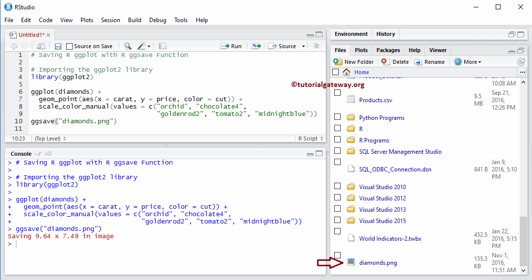
Now, to save this plot, we use ggsave().

# A simple save to a PNG file
ggsave(filename = "figures/toothgrowth_plot.png", plot = p_tooth)

Note: This command assumes you have a sub-folder named figures in your RStudio Project. It's a good habit to organize outputs this way.

3. Controlling Your Output: Key ggsave() Arguments

The real power of ggsave() lies in its arguments, which allow you to meet specific publication requirements. Let's explore the most important ones.

The article below provides an excellent overview of both the basic ggsave() function and some best practices for its use.

As you read, the essential arguments to master are:

• filename: The name of the output file. The file extension you use (.png, .pdf, .tiff, .jpeg, .svg) automatically determines the output format.
• plot: The plot object you want to save (e.g., p_tooth).
• width and height: The physical dimensions of the saved plot.
• units: The units for width and height (e.g., "in" for inches, "cm" for centimeters, "mm" for millimeters).
• dpi: "Dots per inch," which sets the resolution for raster formats (like PNG and TIFF). Common values are 300 for high-quality screen display and 600 or higher for print publication.

Let's save our ToothGrowth plot again, but this time as a 6x4 inch TIFF file with a resolution of 600 DPI, a common requirement for print journals.

ggsave(
  filename = "figures/toothgrowth_publication.tiff", 
  plot = p_tooth,
  width = 6, 
  height = 4, 
  units = "in", 
  dpi = 600
)

The following video demonstrates this exact process, emphasizing how these arguments give you precise control over the final output.

4. Vector vs. Raster: Choosing the Right Format

The file extension in filename is not just a label; it tells ggsave() what kind of file to create. There are two main families of image formats:

• Vector Formats (.pdf, .svg): These formats store images as a set of mathematical instructions (e.g., "draw a line from point A to point B"). Their key advantage is infinite scalability. You can zoom in on a PDF or SVG as much as you want, and the lines and text will remain perfectly sharp. This makes them ideal for plots containing text and geometric shapes. Many journals prefer or require PDF figures.

• Raster Formats (.png, .jpeg, .tiff): These formats store images as a grid of colored pixels. They are excellent for complex images like photographs. However, if you enlarge a raster image too much, it will become blurry or "pixelated." The dpi argument is only relevant for these formats, as it determines the density of pixels in the grid.

For most plots you create with ggplot2, a vector format like PDF is an excellent choice because it guarantees high quality at any size. You would typically use a raster format like TIFF if a journal specifically requires it or if your plot contains thousands of semi-transparent data points, where a PDF could become a very large and slow-to-render file.

5. Best Practices for a Reproducible Workflow

Saving plots is part of your overall analysis workflow. Adopting good habits here will make your research more organized and reproducible.

• Organize Your Files: As mentioned, create a figures or outputs sub-directory within your RStudio Project. Save all your plots there. This keeps your project tidy. If you are using the here package, you can construct a robust path like this: here::here("figures", "my_plot.png").

• Use Descriptive Filenames: Name your files clearly. figure1_scatterplot_bp_vs_weight.pdf is much more informative than plot.pdf. The snake_case naming convention (all lowercase, with words separated by underscores) is a common and recommended standard in the R community.

The Tilburg Science Hub article you looked at earlier contains excellent advice on this.

Conclusion

You have now completed the entire visualization pipeline, from raw data to a publication-ready figure file. With ggsave(), you have the power to export your carefully crafted ggplot2 plots with the precise specifications needed for any medium, be it a journal article, a poster, or a slide presentation.

Key Takeaways:

• Always check the figure submission guidelines of your target publication for requirements on file format, dimensions (width, height), and resolution (dpi).
• ggsave() is the standard function for saving ggplot2 plots. Best practice is to save your plot to a variable first.
• Use the width, height, units, and dpi arguments in ggsave() to gain precise control over the output.
• Choose the right file format for the job. Vector formats like PDF (.pdf) are generally preferred for their scalability and sharp rendering of lines and text.
• Maintain an organized project by saving plots to a dedicated figures directory and using descriptive, consistent filenames.

Preview of the Next Lesson:
Saving plots as individual files is essential, but often you need to integrate them into a larger document that includes your narrative, code, and tables. In the next module, we will dive into R Markdown. You will learn how to weave your text, R code, and ggplot2 visualizations together into a single, cohesive, and fully reproducible report that can be exported as HTML, PDF, or Word documents. This will be a major step towards producing complete data analysis projects.