Enhance Plot Aesthetics with `labs()` and `theme()`

1. The First Step to Clarity: Labeling with labs()

A plot without clear labels is like a map without a key. The viewer doesn't know what they're looking at or why it's important. ggplot2 automatically generates labels from your variable names, but these are rarely suitable for a final report (e.g., body_mass_g should be "Body Mass (g)").

The labs() function provides a single, consistent interface to set all the text on your plot. This includes the main title, a subtitle for more context, a caption for data sources or notes, and labels for all aesthetics (like x, y, color, fill, etc.).

Let's start with the box plot of penguin body mass from our previous lesson.

library(tidyverse)



# If you don't have this plot object, you can recreate it with:
p <- ggplot(data = penguins, mapping = aes(x = species, y = body_mass_g)) +
  geom_boxplot()

Now, let's add professional labels.

p +
  labs(
    title = "Body Mass Distribution Across Penguin Species",
    subtitle = "Data collected from Palmer Station, Antarctica",
    x = "Penguin Species",
    y = "Body Mass (g)",
    caption = "Source: Palmer Penguins R package"
  )

The video below offers a great demonstration of how the labs() layer works to quickly improve a plot.

As you can see, labs() is straightforward and immensely powerful. It’s the first and most important step in making your plot understandable to a wider audience.

2. A New Look: Applying Themes

While labs() controls the text content, the overall visual style—background, grid lines, fonts, colors—is controlled by the theme. ggplot2 has a default theme with a gray background and white grid lines. While functional, you might prefer a different style for your publication.

ggplot2 comes with several built-in themes that you can apply with a single line of code. Some of the most common are:

• theme_bw(): A classic "black and white" theme with a white background and gray grid lines.
• theme_minimal(): A very clean theme that removes the background and most axis lines.
• theme_classic(): A traditional scientific plot theme with x and y axis lines but no background or grid lines.

Let's apply theme_minimal() to our labeled penguin plot. It's often favored for its clean look in modern publications.

# Our plot with labels
p_labeled <- p +
  labs(
    title = "Body Mass Distribution Across Penguin Species",
    subtitle = "Data collected from Palmer Station, Antarctica",
    x = "Penguin Species",
    y = "Body Mass (g)",
    caption = "Source: Palmer Penguins R package"
  )




# Now, add a new theme
p_labeled +
  theme_minimal()

Instantly, the plot feels lighter and less cluttered. Applying a pre-built theme is the quickest way to dramatically change your plot's appearance.

3. Taking Full Control: Customizing with theme()

Pre-built themes are a great starting point, but for true "publication-quality" work, you need to control every detail. This is done with the theme() function. You can use it to modify any of the hundreds of individual elements that make up a plot.

Conceptually, there are two types of arguments you'll use inside theme():

1. Arguments that take a direct value: For example, legend.position = "top" moves the legend to the top.
2. Arguments that take an element function: Most arguments correspond to a visual element on the plot (text, lines, or rectangles). You modify them using one of these functions:
   • element_text(): For all text elements (titles, labels, etc.).
   • element_rect(): For all rectangular elements (backgrounds, borders).
   • element_line(): For all line elements (grid lines, axis lines).
   • element_blank(): To remove an element completely.

The video you watched earlier gives a superb explanation of this system.

A Practical Example: Polishing Our Plot

Let's put this knowledge into practice. We'll start with our plot using theme_minimal() and then make specific adjustments to achieve a polished final version, much like the example below.

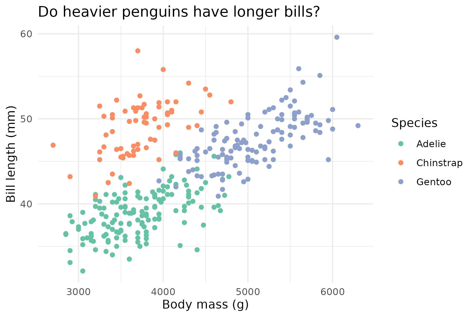
Here's our goal:

1. Make the main title bold and centered.
2. Move the legend to the top.
3. Remove the minor grid lines to reduce clutter.

Let's build the code step-by-step.

# Our base plot with labels and a minimal theme
p_final <- p_labeled + theme_minimal()




# Now, let's add a custom theme layer
p_final +
  theme(



    # 1. Modify the plot title
    plot.title = element_text(face = "bold", hjust = 0.5),




    # 2. Move the legend to the top
    legend.position = "top",
    



    # 3. Remove minor grid lines
    panel.grid.minor = element_blank()
  )

Let's break down the theme() call:

• plot.title = element_text(...): We target the plot.title element. Inside element_text(), we set face = "bold" to make it bold and hjust = 0.5 to center it horizontally (0 is left, 1 is right).
• legend.position = "top": This is a direct argument. We simply provide the position as a character string.
• panel.grid.minor = element_blank(): We target the minor grid lines and use element_blank() to remove them entirely.

Cédric Scherer's comprehensive ggplot2 tutorial is an excellent resource for exploring the vast possibilities of the theme() function. It's a perfect reference to bookmark for future use.

By combining a base theme with specific theme() modifications, you gain complete control over your plot's appearance, allowing you to meet the specific style guides of journals or your own aesthetic preferences.

Conclusion

You have now moved beyond just displaying data to thoughtfully designing a visualization. By mastering labs() and theme(), you have the power to transform a basic R plot into a clear, professional, and publication-quality graphic. This is a fundamental skill for anyone doing data analysis for research.

Key Takeaways:

• Use labs() to control all textual elements of your plot, including titles, subtitles, captions, and axis/legend labels.
• Apply a built-in theme like theme_minimal() or theme_bw() for a quick and significant style change.
• Use the theme() function for fine-grained control over individual non-data elements.
• Inside theme(), modify text with element_text(), rectangles with element_rect(), lines with element_line(), and remove elements with element_blank().

Preview of the Next Lesson:
We've customized the labels and the general theme, but what about the specific colors, shapes, or sizes that ggplot2 assigned to our data? For instance, how could you ensure that the "Adelie" species is always represented by a specific shade of orange? In our next lesson, we will dive into scale functions, which give you precise control over how data values are mapped to visual aesthetics.