Visualizing Distributions

1. Histograms: Visualizing Frequencies

A histogram is the most direct way to see the shape of a continuous variable's distribution. It works by grouping the data into a series of intervals, or "bins," and then plotting the number of observations that fall into each bin as a bar. This gives you an immediate sense of the data's central tendency, spread, and skewness.

In a clinical context, you might use a histogram to check the distribution of patient ages, baseline blood pressure readings, or scores on a psychological scale. This initial check is vital for assessing assumptions of statistical models, such as normality.

The "R for Data Science" text provides a concise introduction to visualizing distributions of numerical variables.

Let's create our first histogram. We'll use the penguins dataset from the palmerpenguins package, which is loaded with tidyverse. First, ensure you have tidyverse loaded.

library(tidyverse)



# The palmerpenguins package is also loaded with tidyverse.
# Let's inspect the data first.
glimpse(penguins)

Now, let's visualize the distribution of penguin body mass.

ggplot(data = penguins, mapping = aes(x = body_mass_g)) +
  geom_histogram()

You might see a message like: stat_bin() using bins = 30. Pick better value with binwidth. This is ggplot2's way of telling you that it chose a default number of bins (30), but that you should always experiment. The choice of bin width can dramatically change the plot's appearance.

The following video from yuzaR Data Science explains this concept very clearly and shows how to adjust the bins.

As the video explains, using binwidth is often better because it's specified in the units of your data (in this case, grams). Let's try a few different binwidths to see the effect.

# A larger binwidth (may hide features)
ggplot(data = penguins, mapping = aes(x = body_mass_g)) +
  geom_histogram(binwidth = 500)




# A smaller binwidth (may be too noisy)
ggplot(data = penguins, mapping = aes(x = body_mass_g)) +
  geom_histogram(binwidth = 50)




# A more reasonable binwidth
ggplot(data = penguins, mapping = aes(x = body_mass_g)) +
  geom_histogram(binwidth = 200, color = "white", fill = "steelblue")

In the last example, I've also set color to outline the bars and fill to change their color, making the plot easier to read. Notice how a binwidth of 200 reveals a bimodal distribution (two peaks), a feature that was less clear with other choices. In a research setting, such a pattern might suggest the presence of two distinct subgroups in your data (e.g., males and females).

2. Density Plots: A Smoother View

A density plot, created with geom_density(), can be thought of as a smoothed version of a histogram. It computes an estimate of the underlying probability distribution of the data. The analogy from "R for Data Science"—imagining a spaghetti noodle draped over the bars of a histogram—is a helpful way to picture this.

Density plots are excellent for observing the overall shape of a distribution, especially its modality (number of peaks), without being distracted by the choice of bins.

ggplot(data = penguins, mapping = aes(x = body_mass_g)) +
  geom_density()

The real power of density plots comes from comparing distributions between different groups. For instance, we can check if the distribution of body mass differs across the three penguin species. We do this by mapping the species variable to an aesthetic like color or fill.

# Using 'color' to draw different lines for each species
ggplot(data = penguins, mapping = aes(x = body_mass_g, color = species)) +
  geom_density(linewidth = 1) # linewidth makes the lines thicker




# Using 'fill' to create shaded areas. 'alpha' adds transparency.
ggplot(data = penguins, mapping = aes(x = body_mass_g, fill = species)) +
  geom_density(alpha = 0.5)

This is a powerful technique. In a clinical trial, you could use this exact method to visually compare the distribution of an outcome variable between the placebo, treatment A, and treatment B groups. The textbook "Mastering Health Data Science Using R" provides a relevant example.

3. Box Plots: Summarizing and Comparing Distributions

While histograms and density plots show the full shape, a box plot (geom_boxplot()) provides a compact summary of a distribution. It is constructed from five key statistics:

• The median (the line inside the box).
• The first quartile (Q1) and third quartile (Q3) (the bottom and top edges of the box). The box itself represents the interquartile range (IQR), which contains the middle 50% of the data.
• The whiskers, which typically extend to 1.5 times the IQR from the edge of the box.
• Outliers, shown as individual points beyond the whiskers.

"R for Data Science" provides a clear diagram explaining this structure.

Box plots are particularly effective for comparing the distribution of a continuous variable across different categories. Let's compare penguin body mass across species again.

ggplot(data = penguins, mapping = aes(x = species, y = body_mass_g)) +
  geom_boxplot()

This plot instantly reveals several key insights:

• Adelie penguins have the lowest median body mass.
• Gentoo penguins have the highest median body mass and the greatest spread (larger IQR).
• The Chinstrap distribution is more compact than the others.

This is one of the most common plots in scientific papers for comparing groups, for example, showing blood pressure measurements (y) for different treatment groups (x).

4. Choosing the Right Chart and Combining Layers

You now have three tools to visualize distributions. How do you choose?

As the flowchart suggests:

• For one group, use a histogram or density plot if you need to see the detailed shape. Use a box plot for a quick summary.
• For 2-5 groups, use side-by-side box plots for a quick comparison of summaries. Use overlaid density plots (or violin plots, which we haven't covered but combine a box plot and a density plot) to see detailed shape differences.

Sometimes, the best visualization combines multiple geoms. A common and highly informative plot overlays the raw data points on top of a box plot. This gives you both the summary (from the box plot) and a sense of the sample size and raw distribution (from the points). We use geom_jitter() instead of geom_point() to add a small amount of random noise to prevent points from overlapping perfectly.

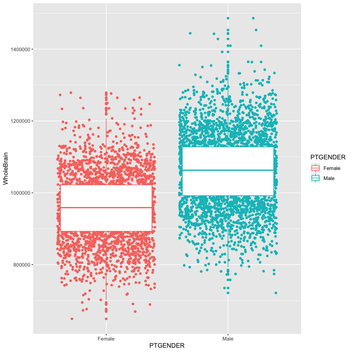
Let's create a similar plot for our penguins data.

ggplot(data = penguins, mapping = aes(x = species, y = body_mass_g, color = species)) +
  geom_boxplot(alpha = 0) + # make boxplot transparent
  geom_jitter(width = 0.2, alpha = 0.7) + # add jittered points
  guides(color = "none") # hide the legend since the x-axis is enough

This combined plot is often superior to either plot alone, aligning with your goal of creating an "extravagant build" that is both informative and visually appealing.

Conclusion

In this lesson, you've added three essential visualization types to your R toolkit. You can now go beyond simple relationships to explore and compare the fundamental distributions of your data. This is a cornerstone of robust data analysis and a critical step in preparing for formal statistical testing.

Key Takeaways:

• geom_histogram() is your tool for seeing the binned frequency distribution of a single numeric variable. Always experiment with binwidth.
• geom_density() provides a smoothed view of a distribution's shape and is excellent for comparing distributions between groups by mapping a category to color or fill.
• geom_boxplot() offers a compact five-number summary of a distribution and is the standard for comparing a numeric variable across multiple categories.
• Combining geoms, like geom_boxplot() with geom_jitter(), can create richer, more informative plots.

Preview of the Next Lesson:
Our plots are becoming quite powerful, but they still have default ggplot2 titles and labels. To make them truly "publication-quality," you need full control over their appearance. In the next lesson, we will focus on customizing plots by modifying titles, axis labels, and overall themes using labs() and theme().