"Crafting Visualizations with `ggplot2`"

1. Scatter Plots: Visualizing Relationships

Scatter plots are the workhorse for exploring the relationship between two continuous, or numeric, variables. In a research context, you would use a scatter plot to visually inspect for correlation between two measurements (e.g., anxiety scores vs. depression scores) before performing a formal statistical test. The geom for this is geom_point().

The basic structure is to map your two continuous variables to the x and y aesthetics and then add the geom_point() layer.

The following reading from the "Stats and R" blog provides a clear, practical guide to building these common plots. We'll start with the scatter plot section.

Let's put this into practice. We'll use the mpg dataset, which is included with ggplot2 and contains fuel economy data for various cars. First, make sure you have the tidyverse loaded, which includes ggplot2.

library(tidyverse)




# A basic scatter plot
ggplot(data = mpg, mapping = aes(x = displ, y = hwy)) +
  geom_point()

This code creates a scatter plot showing the relationship between engine displacement (displ) and highway miles per gallon (hwy). As you'd expect, cars with larger engines tend to have lower fuel efficiency.

Recapping Mapping vs. Setting

A common task is to make a plot clearer by using aesthetics like color. Remember the key distinction from our last lesson:

• Mapping an aesthetic (inside aes()) makes the visual property represent a variable.
• Setting an aesthetic (outside aes()) gives all elements a fixed visual property.

Let's see this in code. To make all points blue, we set the color inside geom_point().

# Setting the color of all points to blue
ggplot(data = mpg, mapping = aes(x = displ, y = hwy)) +
  geom_point(color = "blue")

To make the color of the points represent the car's class, we map the color aesthetic inside aes(). ggplot2 automatically handles the colors and adds a legend.

# Mapping the color of points to the 'class' variable
ggplot(data = mpg, mapping = aes(x = displ, y = hwy, color = class)) +
  geom_point()

2. Line Plots: Showing Trends

Line plots are ideal for visualizing how a variable changes over a continuous range, most often time. In clinical studies, you might use a line plot to track a patient's response to treatment over several weeks. The geom for this is geom_line().

The following video from R Programming 101 demonstrates creating a simple line plot and shows how to combine geom_point() and geom_line(), a very common technique to show both the individual data points and the overall trend.

Let's apply this using the economics dataset, which tracks US economic data over time. We will plot the number of unemployed people (unemploy) against the date.

# A simple line plot
ggplot(data = economics, mapping = aes(x = date, y = unemploy)) +
  geom_line()

The line clearly shows the fluctuations in unemployment over several decades. geom_line() works by connecting the data points in order of their x value, which is why it's perfect for time series data. If you were to use geom_line() on the mpg scatter plot from before, you would get a nonsensical scribble as it tries to connect all the points from left to right.

3. Bar Charts: Comparing Groups and Counts

Bar charts are essential for comparing values across different categories. A frequent point of confusion is that ggplot2 has two related geoms:

1. geom_bar(): Use this when you want to visualize the count of observations in each category. You only need to provide an x aesthetic; ggplot2 calculates the y value (the count) for you.
2. geom_col() (for columns): Use this when your data already contains a column with the value you want to plot as the bar height. You must provide both x and y aesthetics.

Using geom_bar() for Counts

Let's use geom_bar() to see how many cars of each class are in the mpg dataset.

Here is the code in action:

# Bar chart showing counts of cars in each class
ggplot(data = mpg, mapping = aes(x = class)) +
  geom_bar()

A more powerful use of bar charts is to visualize the relationship between two categorical variables. We can do this by mapping the fill aesthetic.

The following video provides an excellent walkthrough of this process, including how to use the position argument to control how the bars are arranged.

Let's try this by looking at the class of car, broken down by drive type (drv).

• Stacked (default): Shows the composition of each class.

  ggplot(data = mpg, mapping = aes(x = class, fill = drv)) +
    geom_bar() # position = "stack" is the default
  

• Dodged: Places bars side-by-side, which is better for comparing the counts of drive types within each class.

  ggplot(data = mpg, mapping = aes(x = class, fill = drv)) +
    geom_bar(position = "dodge")
  

• Filled: Each bar goes to 100%, showing the proportion of each drive type within a class. This is excellent for comparing compositions across groups of different sizes.

  ggplot(data = mpg, mapping = aes(x = class, fill = drv)) +
    geom_bar(position = "fill")
  

Using geom_col() for Pre-calculated Values

Now, what if you don't want to plot counts, but instead a summary value you've already calculated, like a mean? This is where geom_col() is used.

First, you need to calculate the summary statistic. We can use dplyr functions you've already learned (group_by and summarise) to find the average city mileage (cty) for each car class.

# 1. Create a summary table
mpg_summary <- mpg %>%
  group_by(class) %>%
  summarise(avg_cty = mean(cty))




# Print the summary table to see what it looks like
print(mpg_summary)

Now, we can plot this mpg_summary data frame using geom_col(), mapping class to x and our new avg_cty column to y.

# 2. Plot the summary table with geom_col()
ggplot(data = mpg_summary, mapping = aes(x = class, y = avg_cty)) +
  geom_col()

This plot directly visualizes the average mileage for each class, a task for which geom_bar() would be inappropriate.

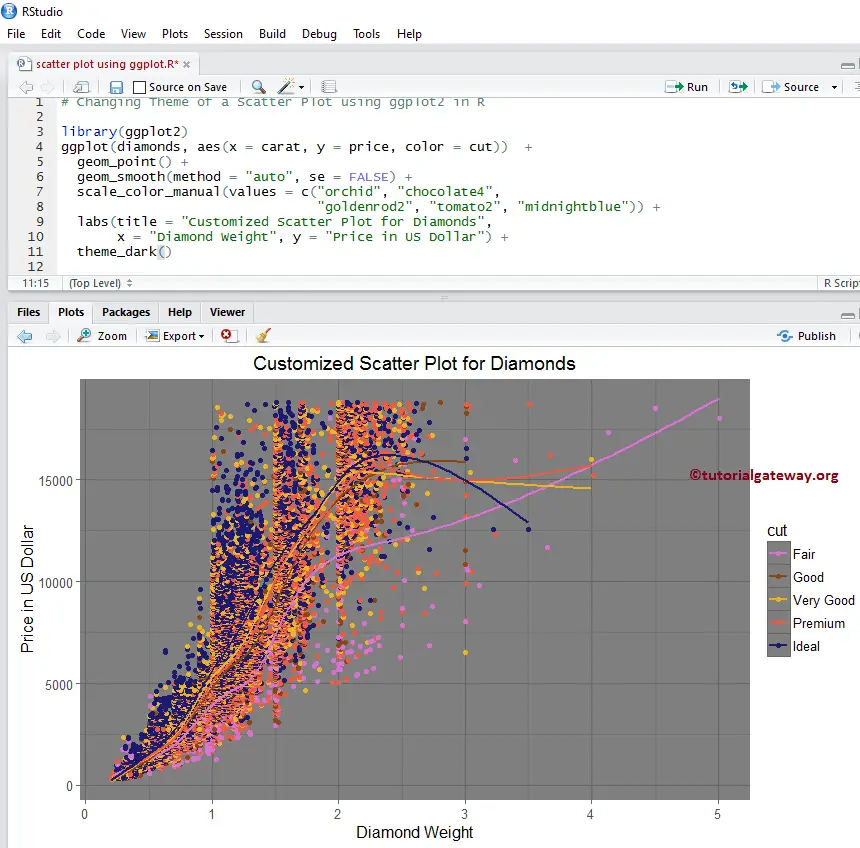
This workflow—summarizing your data with dplyr and then plotting the result with ggplot2—is an extremely common and powerful pattern in data analysis. The Customized Scatter Plot for Diamonds image below shows a more complex example of this process, combining a scatter plot, color mapping, and smoothing lines, all customized to create a publication-ready graphic.

Conclusion

In this lesson, you've translated the theory of the Grammar of Graphics into practical skill by creating three essential plot types. You now have the tools to visualize relationships, trends, and group comparisons—the building blocks of visual data exploration in any research project.

Key Takeaways:

• geom_point() creates scatter plots to show the relationship between two numeric variables.
• geom_line() creates line plots, which are ideal for visualizing trends over a continuous variable like time.
• Geoms can be layered; geom_point() + geom_line() is a common combination.
• geom_bar() is used for plotting the counts of a categorical variable.
• geom_col() is used for plotting pre-calculated values (like means) for different categories.
• The position argument in geom_bar() (dodge, fill, stack) is critical for effectively comparing multiple categorical variables.

Preview of the Next Lesson:
We have focused on relationships between variables (geom_point(), geom_line()) and counts of categories (geom_bar()). The other fundamental task in data exploration is to understand the distribution of a single variable. In our next lesson, we will explore geoms designed for this purpose, including histograms (geom_histogram()), density plots (geom_density()), and box plots (geom_boxplot()).