Grammar of Graphics Fundamentals

1. The Philosophy of Layered Graphics

At its core, the Grammar of Graphics proposes that a statistical graphic is a mapping of variables in your data to aesthetic properties (like position, color, or shape) of geometric objects (like points, lines, or bars).

This is analogous to how language works. We combine elements like nouns and verbs according to grammatical rules to form meaningful sentences. Similarly, ggplot2 allows us to combine layers like data, aesthetics, and geoms according to the Grammar of Graphics to build meaningful plots.

The video below from the R Programming 101 channel offers an excellent high-level introduction to this idea, focusing on the three most important components.

As the video mentioned, we will focus on these three essential layers. However, it's useful to see how they fit into the complete seven-layer grammar.

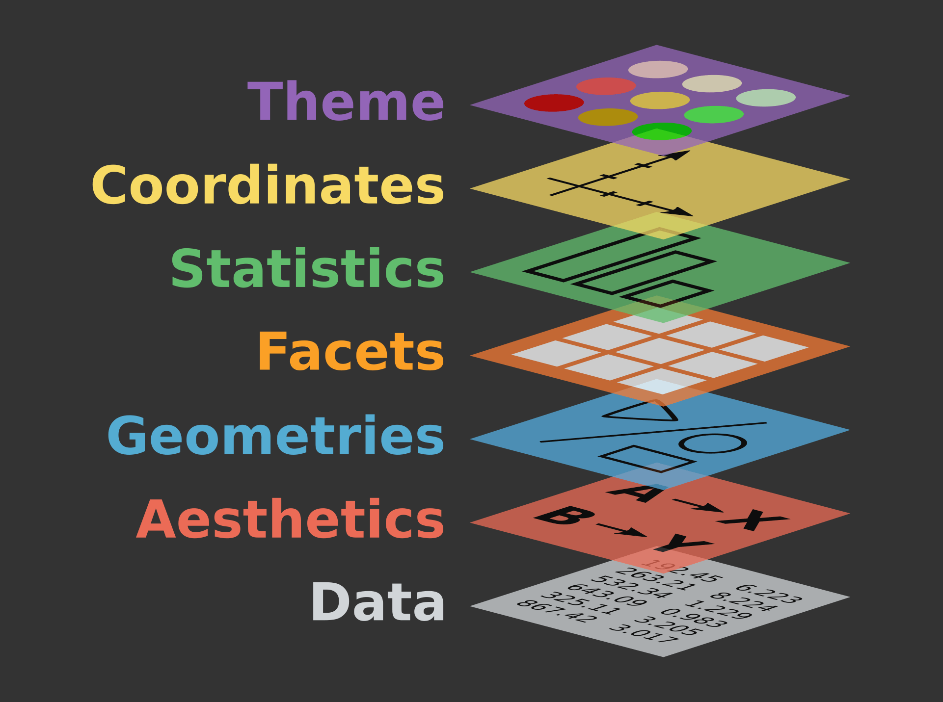
2. The Three Essential Components

To create any plot with ggplot2, you must define three key things. Let's explore each one.

Let's break these down further.

a. Data

This is the most straightforward component. Every plot begins with a dataset, which in R is almost always a data frame or a tibble. This data frame contains the variables you wish to visualize.

b. Aesthetics (aes)

Aesthetics are the visual properties of the plot that can be controlled. This is where you connect, or map, the variables from your dataset to visual elements on the plot. Common aesthetics include:

• x and y (the position on the axes)
• color (the outline of a shape)
• fill (the interior of a shape)
• size (the size of points or thickness of lines)
• shape (the shape of points)
• alpha (the transparency)

The concept of mapping is crucial. You are not telling ggplot2 to "make the points blue." You are telling it to "let the color of the points represent the species variable." ggplot2 then automatically assigns a unique color to each species and creates a legend for you.

This image provides a perfect illustration of mapping:

c. Geometries (geom)

Geometries are the geometric objects that are used to represent your data on the plot. The geom you choose determines the type of plot you create. For example:

• geom_point() creates a scatter plot by drawing a point for each observation.
• geom_line() creates a line graph, often used for time series.
• geom_bar() creates a bar chart.

You can even combine multiple geoms in a single plot, for example, by overlaying a line on top of points.

3. Building a Plot, Layer by Layer

Now, let's see how these three components come together in code. The basic template for a ggplot2 call is:

ggplot(data = YOUR_DATA, mapping = aes(x = VARIABLE_1, y = VARIABLE_2)) +
  geom_FUNCTION()

Notice how the data and mapping are defined inside the main ggplot() function, and then the geom layer is added using a + sign. This additive, layered approach is what makes ggplot2 so flexible.

The following reading walks you through the process of building a plot step-by-step, showing how each layer contributes to the final graphic.

4. Mapping vs. Setting Aesthetics

A common point of confusion for new ggplot2 users is the difference between mapping an aesthetic to a variable and setting it to a fixed value.

• Mapping: When you want a visual property to represent a variable from your data, you put the mapping inside the aes() function. For example, aes(color = region) tells ggplot2 to assign a different color to each unique value in the region column. ggplot2 automatically creates a legend.
• Setting: When you want to apply a visual property to all elements uniformly, you specify it as an argument to the geom_*() function, outside of aes(). For example, geom_point(color = "blue") makes all points blue. The color does not represent any data and no legend is created.

The distinction is critical for creating the exact visual you intend. The following reading clarifies this with clear examples.

5. The Complete Grammar

While we have focused on the three essential layers, the full grammar provides a comprehensive system for describing any plot. The canonical book R for Data Science provides a concise summary of this theoretical framework. Understanding this will cement the concepts we've discussed today.

This systematic view is what makes ggplot2 so powerful. Once you are fluent in this grammar, you are not limited to pre-packaged plot types; you have the building blocks to invent your own visualizations to best tell the story in your data.

Conclusion

In this lesson, you have learned the "why" behind ggplot2—the Grammar of Graphics. By deconstructing plots into independent, combinable layers, this system provides an incredibly powerful and flexible foundation for data visualization. Your understanding of this framework is the first and most important step toward creating the publication-quality graphics needed for your research goals.

Key Takeaways:

• Grammar of Graphics: A theoretical framework that defines plots as a combination of independent layers.
• Three Essential Components: Every ggplot2 graphic requires data (a data frame), aes (mappings of variables to visual properties), and at least one geom (the geometric objects that represent the data).
• Layered Syntax: Layers are combined using the + operator. Data and aesthetic mappings are typically defined globally in ggplot(), and geoms are added as separate layers.
• Mapping vs. Setting: Mappings connect aesthetics to data variables and are placed inside aes(). Settings apply a fixed aesthetic to all objects and are placed outside aes(), within a geom function.

Preview of the Next Lesson:
With this theoretical foundation in place, we will move on to the practical application. In the next lesson, you will use your knowledge of data, aesthetics, and geoms to create some of the most common and useful plot types for research: scatter plots, line plots, and bar charts.