Knitting R Markdown Documents

The Magic of Knitting

At its heart, "knitting" is the process of turning your .Rmd source file—a mix of text and code—into a polished, self-contained report. In RStudio, this powerful process is made incredibly simple, often boiling down to a single click.

The primary way you'll do this is with the "Knit" button, located at the top of the script editor pane in RStudio. Clicking the small dropdown arrow next to it reveals the different document types you can create.

The true power of R Markdown is that from one single .Rmd source file, you can generate multiple, completely different output files, each tailored for a specific purpose.

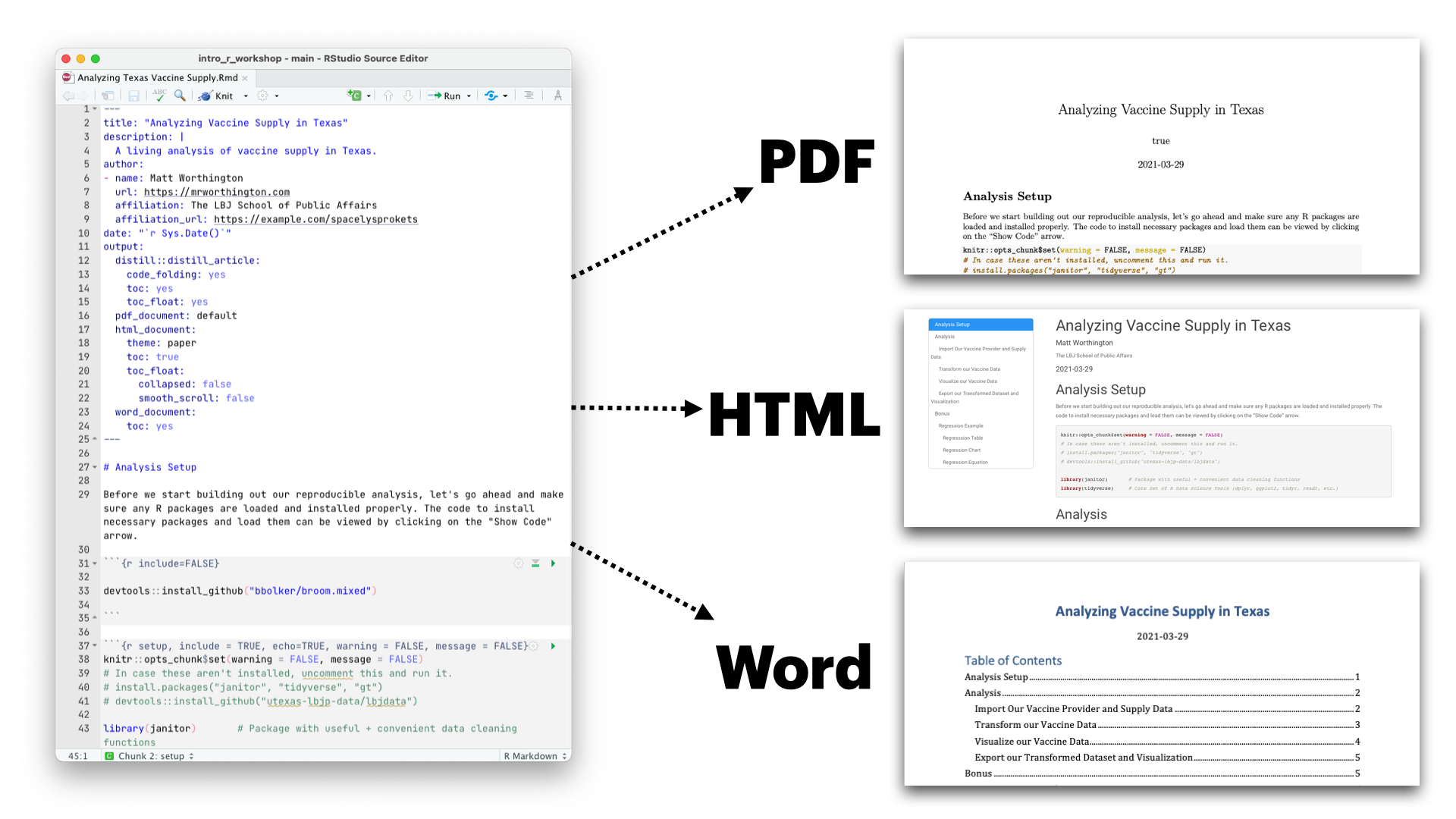
This might seem like magic, but under the hood, RStudio is orchestrating a sophisticated, three-step process. Understanding this process will give you the foundational knowledge you need to troubleshoot issues and customize your outputs effectively.

Demystifying the Process: R Markdown, knitr, and Pandoc

When you click the "Knit" button, RStudio initiates a workflow that involves two key tools working in sequence: knitr and Pandoc.

1. The .Rmd file is passed to knitr: The knitr package (which you've already used for kable()) reads through your file. It executes all the R code in your chunks, captures the results (like tables and plots), and combines them with your narrative text. The output of this step is a plain Markdown (.md) file.
2. The .md file is passed to Pandoc: Pandoc is a universal document converter. It takes the Markdown file generated by knitr and converts it into the final format you specified, such as HTML, Word, or PDF.

This entire sequence is what happens every time you click "Knit". The following reading from "Reproducible Medical Research with R" provides a concise summary of this workflow.

Generating Your First Reports

Now let's put this theory into practice. The most direct way to generate a report is by using the "Knit" button and its dropdown menu. The video below provides a clear, step-by-step demonstration.

While the "Knit" button is convenient, the "official" way to specify the output format is in the YAML header of your .Rmd file. By changing the output: field, you can control what format is generated by default.

For example:

• For an HTML document: output: html_document
• For a Word document: output: word_document
• For a PDF document: output: pdf_document

The following reading provides a short, hands-on exercise where you'll edit the YAML header directly and see the effect.

Handling Common Hurdles

While knitting to HTML and Word is generally seamless, you might encounter a couple of common issues, particularly when generating PDFs or dealing with file paths.

PDF Generation and LaTeX

Knitting to PDF requires an external dependency: a LaTeX distribution. LaTeX is a powerful typesetting system used extensively in academia for producing beautifully formatted documents. If you don't have it installed, knitting to PDF will fail.

The easiest way to install LaTeX for use with R is via the tinytex R package. You can install it with the following commands in your R console:

install.packages("tinytex")
tinytex::install_tinytex()

This can take some time, but you only need to do it once.

For many situations, a practical workaround is to first knit your document to Word and then use Word's "Save as PDF" or "Export to PDF" functionality. This is a very common workflow, especially when collaborating with others who may need the Word document. The video below briefly touches on this exact strategy.

File Path Errors

Another common error occurs when your R Markdown document can't find a file it needs, like a dataset. The knitting process runs in a clean environment, and its "working directory" is by default the location of the .Rmd file itself. If your data file is somewhere else, the process will fail.

This is precisely the problem that the here package, which we covered in Module 1, is designed to solve. By using here::here("data", "my_data.csv") to specify file paths, you create robust links that work both when you're running code interactively and when you are knitting the document. The video above coincidentally runs into this exact error and shows the consequences.

Beyond the Button: Automation with rmarkdown::render()

The "Knit" button is a friendly graphical interface for a powerful underlying function: rmarkdown::render(). Calling this function from the console or from another R script gives you programmatic control over the rendering process.

Why is this useful? It's the key to automation. Imagine you need to generate a monthly report for a clinical trial. Instead of opening the file and clicking "Knit" each month, you could write a small script that calls render(), automatically naming the output file with the current date. This is a fundamental technique in creating reproducible and scalable analysis pipelines.

The resource below explains the render() function and highlights some of its most useful arguments.

Finally, for creating truly publication-quality reports, you can customize the aesthetic appearance of your outputs using templates. For Word documents, you can specify a reference_docx file with pre-defined styles for headings and text. For HTML documents, you can choose different themes and styles. This is a more advanced topic, but the section on "Templates" in the resource you just read provides an excellent starting point for future exploration.

Practice

Take the iris report you created in the previous lesson's practice exercise. If you don't have it, create a new R Markdown file with the content from that exercise.

1. Knit to HTML: Click the "Knit" button or use the dropdown to select "Knit to HTML". Observe the resulting file.
2. Knit to Word: Change the output: field in your YAML header to word_document, or use the dropdown to select "Knit to Word". Examine the .docx file.
3. Knit to PDF (Optional): If you have installed tinytex, try knitting to PDF. If not, open your Word document and use the "Save as PDF" feature.
4. Notice how the plot and table you styled in the previous lesson look in each final document format.

Conclusion

You have now completed the R Markdown workflow, from authoring to output. You can weave together text, code, plots, and tables into a single source document and, with the click of a button, transform it into professional, shareable reports in multiple formats. This is a cornerstone of reproducible research and a skill that will be invaluable in your career.

Key Takeaways:

• The Knit button in RStudio is the simplest way to render an .Rmd file into a report.
• The knitting process involves knitr (to execute code and create a .md file) and Pandoc (to convert the .md file to the final format like HTML, Word, or PDF).
• You can control the output format using the Knit dropdown menu or by editing the output: field in the YAML header.
• Knitting to PDF requires a LaTeX installation, but a common workaround is to knit to Word and then save as PDF.
• The rmarkdown::render() function allows for programmatic rendering, enabling automation of report generation.

Preview of the Next Lesson:
You've just created a valuable, reproducible analysis report. But what happens when you need to make changes? How do you track different versions of your code and narrative? How do you collaborate with a colleague without creating a mess of files like report_final.docx, report_final_v2.docx, and report_final_JohnsEdits.docx? The next module, Version Control with Git and GitHub, will answer these questions, introducing you to the industry-standard tools for managing change and collaboration in software and data analysis projects.