Sorting Data Frames with `arrange()`

1. The Basics: Ascending and Descending Order

The primary function for sorting rows in dplyr is arrange(). By default, it sorts the data based on the column you specify in ascending order (from smallest to largest for numbers, or alphabetically for characters).

To sort in descending order (from largest to smallest), you wrap the column name in the desc() helper function. This is a very common pattern you'll use to find the "top" values in your dataset.

The PsyTeachR book, which we used in the previous lesson, provides a clear, activity-based introduction to these core concepts.

2. Sorting by Multiple Columns

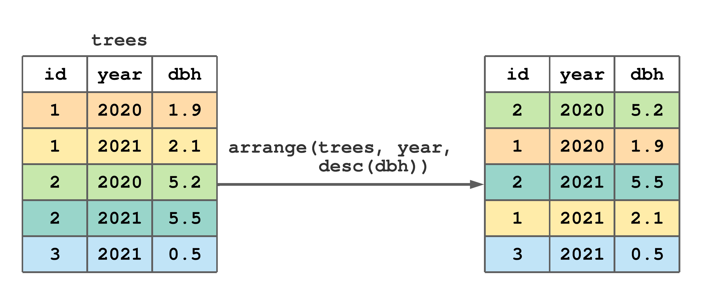
The real power of arrange() becomes apparent when you need to impose a more complex order on your data. In research, you often need to sort by one variable and then use another to "break ties." For example, you might want to list patients by risk group, and within each risk group, sort them by age.

To do this, you simply provide the column names to arrange() in the order of priority. arrange() will sort by the first column, then use the second column to sort any rows that had the same value in the first column, and so on. You can also mix ascending and descending orders for different columns.

The image below provides a perfect visual summary of this process.

Let's see another practical example of this in the PsyTeachR guide.

For a quick video demonstration of this same principle, you can watch this clip.

3. A Note on Missing Values

A practical question that often arises is: where do missing values (NA) go when you sort? In dplyr, the arrange() function has a consistent and convenient rule: NA values are always placed at the end of the sorted output. This is true whether you are sorting in ascending or descending order. This behavior is generally what you want, as it separates the complete cases, which you are often most interested in, from the incomplete ones.

For example, if you arrange(my_data, Age), all rows with a non-missing Age will come first, sorted from youngest to oldest, followed by all rows where Age is NA. If you arrange(my_data, desc(Age)), the non-missing rows will be sorted from oldest to youngest, and again, the rows with NA for Age will be at the very end.

4. Let's Practice

Now it's time to apply arrange() to the blood_storage_modified data frame we created in the last lesson. Open your clinical-trial-practice RStudio Project and create a new R script named 11-arrange-rows.R.

1. Load packages and recreate the data. Add this code to your script and run it to get our starting data frame. This is the same code from the end of the previous lesson.

   library(tidyverse)
   library(medicaldata)
   
   blood_storage_modified <- blood_storage %>%
     mutate(
       PSADensity = PreopPSA / PVol,
       AgeCat = case_when(
         Age < 70 ~ "Under 70",
         Age >= 70 ~ "70 and over"
       ),
       PSARisk = case_when(
         is.na(PreopPSA) ~ "Unknown",
         PreopPSA < 10 ~ "Low",
         PreopPSA <= 20 ~ "Intermediate",
         PreopPSA > 20 ~ "High"
       )
     )
   

2. Your Tasks: Write piped operations to answer the following questions. You don't need to save the results to new objects unless you want to; just printing the sorted output to the console is enough to see the answer.

   • Task 1: Find the Highest PSA Density. Sort the blood_storage_modified data frame to show the patients with the highest PSADensity at the top. Display the top 5 rows of this sorted data frame. Hint: you can pipe your arrange() command into head(5).

   • Task 2: Examine Age Within Risk Groups. Sort the data first by the PSARisk group in its natural alphabetical order ("High", "Intermediate", "Low", "Unknown"). Then, within each risk group, sort the patients by Age from oldest to youngest. This would help you quickly identify the oldest patients in the "High" risk category, for example.

   Click here to see the solution

   
   
   
   # Task 1: Find the patients with the highest PSA Density
   blood_storage_modified %>%
     arrange(desc(PSADensity)) %>%
     head(5)
   
   
   
   
   # --- Output would look something like this ---
   # # A tibble: 5 × 12
   #      PtID Vesinv   [...] AgeCat        PSARisk       PSADensity
   #     <dbl> <fct>        [...] <chr>         <chr>            <dbl>
   # 1   156 No           [...] 70 and over   High             3.21 
   # 2   218 No           [...] Under 70      High             2.17 
   # 3   212 No           [...] 70 and over   High             1.91 
   # 4   360 No           [...] 70 and over   High             1.53 
   # 5   366 No           [...] Under 70      High             1.48 
   # Note: The output has been simplified for clarity. 
   # Also, notice the NAs in PSADensity are not at the top.
   
   
   
   
   
   # Task 2: Sort by risk group, then by age descending
   blood_storage_modified %>%
     arrange(PSARisk, desc(Age))
     
   
   
   
   # If you run this, you will see the data is first grouped by PSARisk ('High', 'Intermediate', etc.)
   # and within each of those blocks, the ages are sorted from largest to smallest.
   

Conclusion

In this lesson, you've added another essential dplyr verb, arrange(), to your data wrangling toolkit. You now have the power to not just select, filter, and create data, but also to order it in a logical and meaningful way. This is a critical step in exploring your data, checking the results of your transformations, and preparing data for presentation.

Key Takeaways:

• arrange() sorts the rows of a data frame based on one or more columns.
• By default, arrange() sorts in ascending order. To sort in descending order, use the desc() function around the column name.
• You can sort by multiple columns to break ties; arrange() uses them in the sequence you provide.
• Missing values (NA) are always sorted to the end of the output, regardless of the sort order.

Preview of the Next Lesson:
We have been building our data transformation skills piece by piece. You can select columns, filter rows, create new variables, and now, sort the entire dataset. In our next lesson, we will learn how to combine these operations with group_by() and summarise(). This will allow you to move from manipulating individual rows to calculating summary statistics for groups within your data—for instance, calculating the average age or median PSA level for each risk category you've created. Sorting is often a useful precursor to these kinds of grouped operations.