Filtering Data with `filter()`

1. The Core Idea: Filtering with Logical Conditions

The filter() function works by applying a logical test to each row of your data. It keeps the rows where the test returns TRUE and discards the rows where it returns FALSE. This simple principle is incredibly powerful.

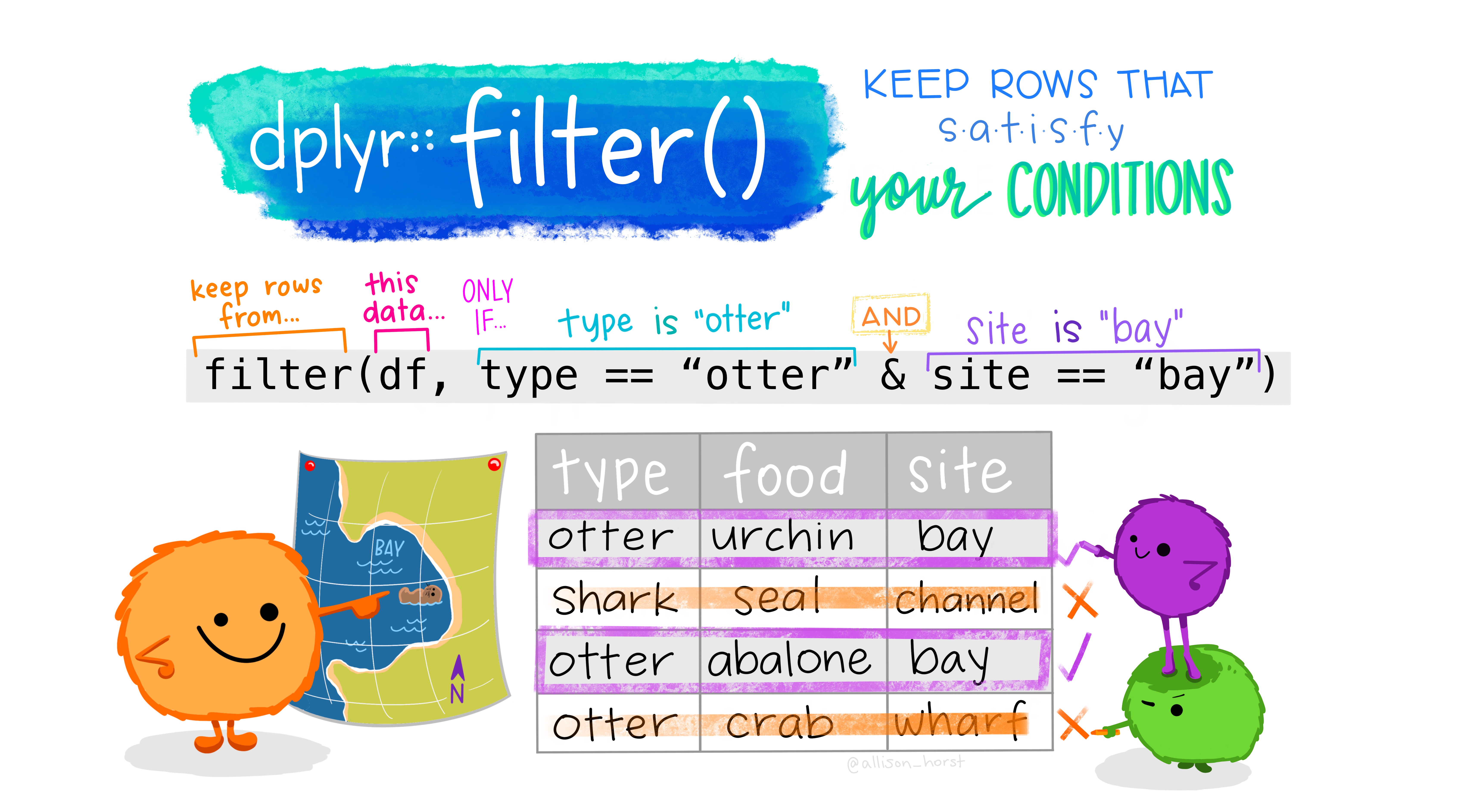
To effectively use filter(), you need to be comfortable writing these logical conditions. A condition is simply an R expression that evaluates to TRUE or FALSE. Let's explore the building blocks for these expressions.

2. Combining Multiple Conditions

Real-world data analysis rarely involves a single condition. You'll more likely need to combine several criteria. For instance, you might need to find patients who are both over 65 years old and belong to a specific treatment group, or patients who have either condition A or condition B.

dplyr allows you to specify multiple conditions within a single filter() call using boolean operators:

• & or a comma (,) for AND: All conditions must be TRUE.
• | for OR: At least one condition must be TRUE.
• ! for NOT: Reverses a condition (e.g., keeps rows that do not match).

The following video provides a clear, step-by-step walkthrough of how to use these operators.

3. Efficient Filtering Helpers

While & and | are powerful, chaining many OR conditions can become cumbersome. For example, to find patients from study sites 'A', 'B', 'D', and 'F', you would have to write:
filter(site == 'A' | site == 'B' | site == 'D' | site == 'F')

dplyr provides more elegant solutions for common scenarios like this.

• %in%: To check if a value is present in a list of options. The example above becomes much cleaner: filter(site %in% c('A', 'B', 'D', 'F')).
• between(): To check if a numeric value falls within a range, inclusive of the endpoints. For example, filter(between(age, 60, 70)) is a more readable equivalent of filter(age >= 60 & age <= 70).

4. A Special Case: Handling Missing Values (NA)

In any real dataset, especially clinical data, you will encounter missing values, represented in R as NA. These values behave in a special way. A logical comparison involving an NA (e.g., NA > 60) doesn't result in TRUE or FALSE; it results in NA. Because filter() only keeps TRUE rows, observations with missing values in the columns you are filtering on will be automatically dropped.

Sometimes you want to explicitly find or remove rows with missing data. To do this, you must use the special function is.na().

• filter(is.na(column_name)) will keep only the rows where column_name is missing.
• filter(!is.na(column_name)) will keep only the rows where column_name is not missing.

This is a critical technique for data cleaning and validation.

5. Let's Practice

Time to apply these concepts. We will continue working with the blood_storage dataset from the medicaldata package.

Open your clinical-trial-practice RStudio Project and create a new R script named 09-filter-rows.R.

1. Load packages and data. Add this code to your script and run it.

   library(tidyverse)
   library(medicaldata)
   
   
   
   
   # We will use the 'blood_storage' dataset
   glimpse(blood_storage)
   

2. Your Tasks: Create new data frames by writing a piped operation for each task below. Inspect the resulting data frame after each step to ensure your code worked as expected.

   • Task 1: Older Male Patients with Recurrence. Create a data frame called older_male_recurrence that contains only male patients (Sex == 1) older than 75 who experienced a recurrence (Recurrence == 1).

   • Task 2: Patients from Specific Age Groups. Create a data frame called specific_age_groups containing patients from RBC age groups 3, 4, or 5. Use the %in% operator for this.

   • Task 3: Patients with Mid-range PSA and No Pre-op Therapy. Create a data frame called mid_psa_no_therapy. This should include patients whose pre-operative PSA (PreopPSA) was between 20 and 50 (inclusive) AND who did not receive pre-operative therapy (PreopTherapy == 0).

   • Task 4: Patients with Missing PSA values. Create a data frame called missing_psa that contains only the patients for whom the PreopPSA value is NA.

   Click here to see the solutions

   
   
   
   # Task 1 Solution
   older_male_recurrence <- blood_storage %>%
     filter(Sex == 1, Age > 75, Recurrence == 1)
   
   glimpse(older_male_recurrence)
   
   
   
   
   # Task 2 Solution
   specific_age_groups <- blood_storage %>%
     filter(RBC.Age.Group %in% c(3, 4, 5))
   
   glimpse(specific_age_groups)
   
   
   
   
   # Task 3 Solution
   mid_psa_no_therapy <- blood_storage %>%
     filter(between(PreopPSA, 20, 50), PreopTherapy == 0)
   
   glimpse(mid_psa_no_therapy)
   
   
   
   
   # Task 4 Solution
   missing_psa <- blood_storage %>%
     filter(is.na(PreopPSA))
     
   glimpse(missing_psa)
   

This practice mirrors the daily work of a data analyst: starting with a broad dataset and progressively narrowing it down to answer specific, targeted questions.

Conclusion

In this lesson, you've added a crucial verb, filter(), to your data transformation vocabulary. You can now subset your data not just by columns (select) but also by rows based on specific, and even complex, criteria. This is the foundation of asking questions and exploring hypotheses with your data.

Key Takeaways:

• filter() keeps rows where a logical condition evaluates to TRUE.
• Use comparison operators (>, <, ==, !=) for basic conditions. Remember to use == for testing equality.
• Combine conditions with boolean operators: , or & for AND, | for OR, and ! for NOT.
• Use helper functions like %in% and between() to write cleaner and more readable code for common filtering tasks.
• Handle missing data explicitly using is.na() to either find or exclude NA values.

Preview of the Next Lesson:
So far, you can select columns and filter rows. But what if you need to calculate a new variable from existing ones, like BMI from height and weight, or categorize patients based on a certain threshold? In our next lesson, we will cover mutate() and case_when(), the dplyr tools that allow you to create new columns and modify existing ones, adding another layer of power to your data wrangling skills.