Grouping and Summarizing Data with `dplyr`

1. The Core Idea: Split-Apply-Combine

Before diving into the code, it's crucial to understand the conceptual workflow. The process of generating a grouped summary involves three steps:

1. Split: The data frame is conceptually split into smaller data frames, one for each unique value of the grouping variable(s) you specify. For instance, if you group by a risk_group column with "Low," "Medium," and "High" values, you are creating three virtual subsets of your data.
2. Apply: A summary function (like mean(), median(), or simply counting the number of rows with n()) is applied independently to each of these subsets.
3. Combine: The results from each subset are collected and combined into a new data frame. This summary data frame will have one row for each group.

This video from Ben Stenhaug provides an excellent conceptual breakdown of how group_by() and summarise() work together to achieve this.

The following diagram illustrates this entire process. The original data frame df is first grouped by cat1, creating three logical groups ('a', 'b', 'c'). Then, summarize() is applied to calculate the average of x, the sum of x, and the count of rows (n()) for each group, producing a new, compact summary table.

2. Syntax and Common Summary Functions

Now let's translate this concept into code. The workflow typically involves piping your data into group_by() and then into summarise().

A common task in clinical research is to summarize patient characteristics. This video from R Programming 101 walks through a practical example using the msleep dataset, demonstrating the full pipeline from data to summary table.

As you saw, summarise() lets you create new columns for your summary data. Inside summarise(), you will use summary functions that collapse a vector of values into a single value. Some of the most common ones are:

• mean(): calculates the average.
• median(): calculates the median.
• sd(): calculates the standard deviation.
• min() and max(): find the minimum and maximum values.
• n(): counts the number of rows in the current group. This function is unique in that it doesn't take any arguments.

Handling Missing Values

A critical point when working with real-world data, especially clinical data, is handling missing values (NA). By default, most summary functions in R will return NA if even one value in the input is NA. This is a safety feature to prevent you from unknowingly calculating a summary on incomplete data. To override this, you must explicitly tell the function to remove missing values before calculation by setting the argument na.rm = TRUE.

The following reading demonstrates why this is so important.

3. Grouping by Multiple Columns

Your research questions might require more granular summaries. For instance, you might want to know the average blood pressure not just for a treatment group, but for males and females within that treatment group. You can achieve this by passing multiple column names to group_by().

data %>% group_by(variable_1, variable_2) %>% summarise(...)

This creates subgroups for every unique combination of variable_1 and variable_2.

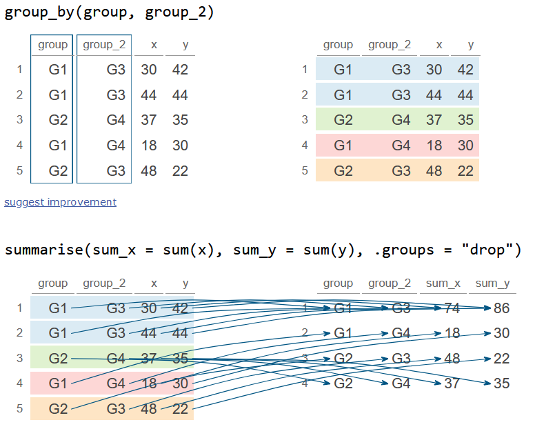
When you summarize data grouped by multiple columns, dplyr has a specific default behavior: it "peels off" only the last grouping variable. The resulting data frame remains grouped by the other variables. This can be useful for subsequent calculations but can also be surprising if you're not aware of it.

The blog post from Andrew Heiss provides an excellent explanation of this behavior and how to control it.

4. Let's Practice

It's time to apply these concepts to our clinical data. Open your clinical-trial-practice RStudio Project and create a new R script named 12-grouped-summaries.R.

1. Load packages and recreate the data. Add this code to your script and run it. This brings in the blood_storage_modified data frame we've been working with.

   library(tidyverse)
   library(medicaldata)
   
   blood_storage_modified <- blood_storage %>%
     mutate(
       PSADensity = PreopPSA / PVol,
       AgeCat = case_when(
         Age < 70 ~ "Under 70",
         Age >= 70 ~ "70 and over"
       ),
       PSARisk = case_when(
         is.na(PreopPSA) ~ "Unknown",
         PreopPSA < 10 ~ "Low",
         PreopPSA <= 20 ~ "Intermediate",
         PreopPSA > 20 ~ "High"
       )
     )
   

2. Your Tasks: Write piped operations to create the following summary tables.

   • Task 1: Patient Counts and PSA by Risk Group. Create a summary table that shows, for each PSARisk group, the number of patients (n), the mean PreopPSA, and the standard deviation of PreopPSA. Name your new columns n_patients, mean_psa, and sd_psa. Remember to handle missing values for the PreopPSA calculations! This is a classic "Table 1" summary found in many clinical studies.

   • Task 2: Prostate Volume by Age and Vesicle Invasion. Create a summary table that shows the median PVol (Prostate Volume) for each combination of AgeCat and Vesinv (seminal vesicle invasion). Group by both variables.

   • Task 3: Find the Deadliest Combination. The sGS column represents the surgical Gleason score, a measure of cancer aggressiveness. Find the combination of PSARisk and sGS that has the highest average PSADensity. Your final output should be a single row showing this combination and its average PSA density. Hint: This will require combining group_by(), summarise(), and arrange() from the last lesson.

   Click here to see the solution

   
   
   
   # Task 1: Patient Counts and PSA by Risk Group
   psa_summary <- blood_storage_modified %>%
     group_by(PSARisk) %>%
     summarise(
       n_patients = n(),
       mean_psa = mean(PreopPSA, na.rm = TRUE),
       sd_psa = sd(PreopPSA, na.rm = TRUE)
     )
   
   print(psa_summary)
   
   
   
   
   # --- Output ---
   # # A tibble: 4 × 4
   #   PSARisk      n_patients mean_psa sd_psa
   #   <chr>             <int>    <dbl>  <dbl>
   # 1 High                 59    33.2   29.7 
   # 2 Intermediate         96    13.4    2.99
   # 3 Low                 187     6.12   1.93
   # 4 Unknown               3   NaN     NA   
   # Note: The 'Unknown' group has NaN/NA because all its PreopPSA values are NA.
   
   
   
   
   
   # Task 2: Prostate Volume by Age and Vesicle Invasion
   pvol_summary <- blood_storage_modified %>%
     group_by(AgeCat, Vesinv) %>%
     summarise(
       median_pvol = median(PVol, na.rm = TRUE),
       .groups = "drop" # Good practice to drop all groups
     )
   
   print(pvol_summary)
   
   
   
   
   # --- Output ---
   # # A tibble: 5 × 3
   #   AgeCat      Vesinv median_pvol
   #   <chr>       <fct>        <dbl>
   # 1 70 and over No            45.9
   # 2 70 and over Yes           46.9
   # 3 Under 70    No            40.4
   # 4 Under 70    Yes           48.6
   # 5 Under 70    NA            39.1
   
   
   
   
   
   # Task 3: Find the deadliest combination
   deadliest_combo <- blood_storage_modified %>%
     group_by(PSARisk, sGS) %>%
     summarise(
       avg_psa_density = mean(PSADensity, na.rm = TRUE),
       .groups = "drop"
     ) %>%
     arrange(desc(avg_psa_density)) %>%
     head(1) # Get the top row
   
   print(deadliest_combo)
   
   
   
   
   # --- Output ---
   # # A tibble: 1 × 3
   #   PSARisk sGS   avg_psa_density
   #   <chr>   <fct>           <dbl>
   # 1 High    10              0.871
   

Conclusion

You have now mastered one of the most powerful and common operations in data analysis: generating grouped summaries. By combining group_by() and summarise(), you can move beyond looking at raw data and begin to quantify patterns and relationships within it.

Key Takeaways:

• The split-apply-combine strategy is a powerful mental model for data summarization.
• group_by() defines the subgroups, and summarise() computes aggregate statistics for those groups.
• Common summary functions include mean(), median(), sd(), min(), max(), and n().
• Always use na.rm = TRUE when summarizing columns that contain missing values (NA).
• You can group by multiple columns to create more granular summaries.
• Be mindful of dplyr's default behavior of leaving "leftover groups" and use ungroup() or .groups = "drop" to control it.

Preview of the Next Lesson:
So far, all our operations have been on a single data frame. However, real-world analysis, especially in research, often requires combining information from multiple sources. For example, you might have one file with patient demographics and another with lab results. In our next lesson, we will learn how to merge two data frames together using dplyr's join functions, starting with the most common one: left_join().