Pivoting Data from Long to Wide with `pivot_wider()`

Introduction

In our previous lesson, you learned how to take "wide" data and reshape it into a "long," tidy format using tidyr::pivot_longer(). This is the standard format required for most analysis and visualization tasks within the Tidyverse. However, the journey of data doesn't always end there. Sometimes, for reporting or presentation, a wide format is actually more intuitive and readable for a human audience.

This lesson focuses on the inverse operation: reshaping data from a long to a wide format. You will learn how to use tidyr::pivot_wider(), a function that is essential for creating summary tables suitable for publications, reports, or theses. Mastering this function will allow you to present the results of your analysis in a clear, condensed format, a crucial skill for communicating your findings in clinical and academic research.

1. The Purpose of Going Wide

While the long format is ideal for computation, the wide format often excels at presentation. Imagine you have a long table showing the average biomarker level for different treatment groups and visit times. For a report, you might prefer a table where each row is a treatment group and each column is a visit, with the biomarker levels in the cells. This is precisely what pivot_wider() is designed to do.

pivot_wider() "widens" data by increasing the number of columns and decreasing the number of rows. It achieves this by taking two key columns from your long data frame:

A "name" column, whose unique values will become the new column headers.
A "value" column, whose values will populate the cells of those new columns.

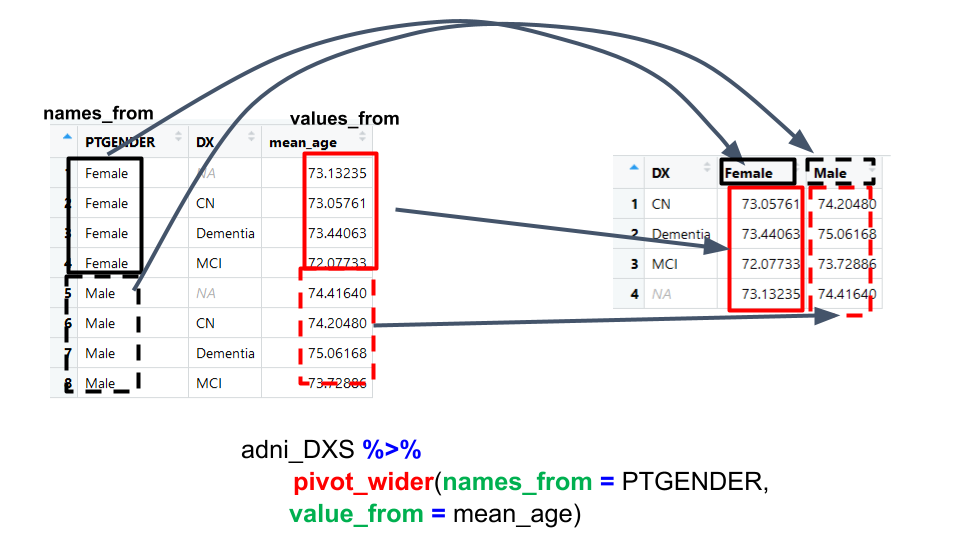
This diagram illustrates the process. Values from a names_from column (here, PTGENDER) become new column headers, and the corresponding data from a values_from column (here, mean_age) fill in the new table.

This image shows how `pivot_wider()` transforms a long data frame. The unique values in the `PTGENDER` column ('Female', 'Male') become new columns. The values from the `mean_age` column are then placed into the appropriate cells.

2. The Mechanics of `pivot_wider()`

The core arguments of pivot_wider() directly correspond to the transformation logic:

names_from: Specifies the column that contains the values you want to turn into new column names.
values_from: Specifies the column that contains the values you want to fill the cells of the new columns.

The video from the "R Programming 101" channel provides a very clear walkthrough of these arguments using a simple, built-in dataset.

Use pivot_wider() to shape your data. R programming from beginners.

This video introduces the concept of widening data and demonstrates the basic syntax of pivot_wider() with its essential arguments.

First, watch the initial segment to understand the goal: the problem. The presenter explains the structure of the long-format Orange dataset and the desired wide-format output. Next, watch the demonstration of the solution. Pay close attention to how the names_from = age and values_from = circumference arguments are used to achieve the transformation.

Now, let's explore this with an example more tailored to your field of clinical research. The "R for health scientists" tutorial demonstrates this in the context of analyzing the ADNI (Alzheimer's Disease Neuroimaging Initiative) dataset.

Manipulating, analyzing and exporting data with tidyverse – R for health scientists

This resource shows a practical, multi-step workflow: summarizing data and then pivoting it into a wide format for easier interpretation. This is a very common pattern in data analysis.

Start by reading the section on reshaping data. This part revisits the concept of tidy data and introduces pivot_longer() and pivot_wider() as the primary tools for changing data shape. Next, carefully study the subsection "Creating wide data". Follow the example closely. Notice how they first create a summary table adni_r_DXS using group_by() and summarize(). This table is in a long format. Then, they apply pivot_wider() to this summary table, specifying names_from = PTGENDER and values_from = mean_age to create a wide, presentation-friendly table.

This example highlights a key use case: pivot_wider() is often the final step after you've calculated summary statistics. You first use dplyr verbs to calculate means, counts, or other metrics, resulting in a long-format summary table. Then, you use pivot_wider() to present those results in a compact, wide table.

3. Let's Practice: Reversing the Pivot

To solidify your understanding, let's return to the patient_biomarkers_long data frame you created in the previous lesson. We will now pivot it back to its original wide format.

Open a new R script in RStudio and name it 16-pivot-wider.R.

Recreate the long dataset. First, load the tidyverse and run the code from our last lesson to create the long-format tibble.

library(tidyverse)




# The original wide data
patient_biomarkers_wide <- tibble::tribble(
  ~patient_id, ~treatment_group, ~biomarker_baseline, ~biomarker_6mo, ~biomarker_12mo,
  "ID01", "Drug A", 25.4, 22.1, 19.8,
  "ID02", "Placebo", 30.1, 31.0, 30.5,
  "ID03", "Drug A", 28.9, 25.6, NA,
  "ID04", "Drug B", 22.5, 20.1, 18.9,
  "ID05", "Placebo", 27.8, 27.5, 28.1
)




# The long-format data you created last time
patient_biomarkers_long <- patient_biomarkers_wide %>%
  pivot_longer(
    cols = starts_with("biomarker_"),
    names_to = "visit",
    values_to = "biomarker_level"
  ) %>%
  drop_na(biomarker_level)




# Let's look at it again
print(patient_biomarkers_long)

Your patient_biomarkers_long table has columns patient_id, treatment_group, visit, and biomarker_level. Each row is a single measurement for a patient at a specific visit.

Your Task: Create a new data frame called patient_biomarkers_wide_again.
- Start with the patient_biomarkers_long data frame.
- Pipe it into pivot_wider().
- Use the visit column to create the new column names.
- Use the biomarker_level column to provide the values for the new columns.
- Finally, print your new patient_biomarkers_wide_again data frame to the console to inspect it. Does it look like the original patient_biomarkers_wide?

Click here to see the solution

patient_biomarkers_wide_again <- patient_biomarkers_long %>%
  pivot_wider(
    names_from = visit,
    values_from = biomarker_level
  )




# Print the result
print(patient_biomarkers_wide_again)

Your resulting tibble should have 5 rows and 5 columns: patient_id, treatment_group, and the three new columns created from the visit values: biomarker_baseline, biomarker_6mo, and biomarker_12mo. You've successfully reversed the pivot_longer() operation! Note that the row for patient ID03 now has an NA in the biomarker_12mo column because that value was missing in the long data.

4. Application in Epidemiology Reporting

The need to create wide summary tables is ubiquitous in medical research. "The Epidemiologist R Handbook" provides another excellent, practical example.

12 Pivoting data – The Epidemiologist R Handbook

This resource explicitly frames pivot_wider() as a tool for creating presentation-ready tables, which directly aligns with your goals.

Please read the section "Long-to-wide". The example starts with a long data frame (df_wide in their code) that contains counts of individuals by age category and gender. While this format is great for plotting with ggplot2, the authors note it's "not ideal for presentation in a table." They then use pivot_wider() to transform it into a much more reader-friendly table where gender becomes the columns. Pay attention to the id_cols argument, which explicitly marks columns that should be kept as unique identifiers for each row.

This example reinforces that data shaping isn't about finding one "correct" format, but about choosing the right format for the task at hand: long for analysis, and often wide for reporting.

Conclusion

You have now added pivot_wider() to your data wrangling toolkit, completing the fundamental pair of reshaping functions in tidyr. You understand not only how to convert data from a long to a wide format but also why and when this is a necessary step, particularly for communicating your findings. Being able to seamlessly move between long and wide formats gives you complete control over the structure of your data.

Key Takeaways:

Purpose: pivot_wider() is used to convert data from a long to a wide format, which is often better for human-readable summary tables in reports.
Mechanism: It works by taking values from a names_from column to create new column headers, and populating those new columns with data from a values_from column.
Inverse Operation: pivot_wider() is the direct opposite of pivot_longer().
Common Workflow: A frequent analysis pattern is to use dplyr::group_by() and dplyr::summarise() to calculate statistics, and then use pivot_wider() to present those statistics in a compact table.

Preview of the Next Lesson:
So far, we have been using functions provided by R packages like dplyr and tidyr. In the next lesson, we will take a significant step towards more powerful and customized programming by learning how to write your own functions. This will enable you to encapsulate repetitive code, make your analyses more modular, and solve problems for which no off-the-shelf function exists.

Recommended resources