Reshaping Data with `pivot_longer()`

Introduction

In our last lesson, we focused on cleaning data by strategically removing rows with missing values using tidyr::drop_na(). This is a crucial step in preparing a dataset for analysis. Today, we shift our attention from the content of our data to its fundamental structure. Real-world data, especially from clinical or experimental settings, is often organized for easy data entry rather than for analysis, which can make your work much harder than it needs to be.

This lesson introduces a powerful data reshaping technique. You will learn how to transform data from a "wide" format, where individual observations are spread across multiple columns, into a "long" or "tidy" format, where each observation has its own row. This is one of the most common and important data wrangling tasks you will perform. Mastering this skill is essential for analyzing repeated-measures data (like patient follow-ups over time) and for leveraging the full power of analysis and visualization tools like dplyr and ggplot2. Our focus will be on the tidyr::pivot_longer() function, a cornerstone of the Tidyverse.

1. The Principle of Tidy Data

Before we start reshaping data, it's essential to understand the goal. In the Tidyverse philosophy, the goal is to create tidy data. A dataset is considered tidy if it adheres to three simple, interrelated rules:

Each variable must have its own column.
Each observation must have its own row.
Each value must have its own cell.

The "RichardOnData" YouTube channel provides a concise and clear explanation of these principles.

Tidying Data in R with "tidyr" | R Tutorial (2020)

This video introduces the core concepts of tidy data, using simple tables to illustrate what makes a dataset tidy versus untidy.

Please watch the segment from the beginning of the discussion on tidy data. Pay close attention to the three rules and how the example tables either follow or violate them.

Data that violates these rules is often in a "wide" format. For instance, imagine a clinical trial where a patient's blood pressure is measured at three different visits. A wide format might have columns named bp_visit1, bp_visit2, and bp_visit3. This violates Rule #1, because bp_visit1, bp_visit2, and bp_visit3 aren't three separate variables. They are three values of a single "blood pressure" variable, corresponding to another "visit" variable.

The tidy, or "long," format would have three columns: patient_id, visit, and blood_pressure. Each row would represent a single observation of one patient at one visit. This structure is far more flexible for analysis. For example, you could easily plot blood pressure over time or calculate the average change between visits.

2. From Wide to Long with `pivot_longer()`

The function tidyr::pivot_longer() is designed specifically to solve this problem. It "lengthens" data by decreasing the number of columns and increasing the number of rows.

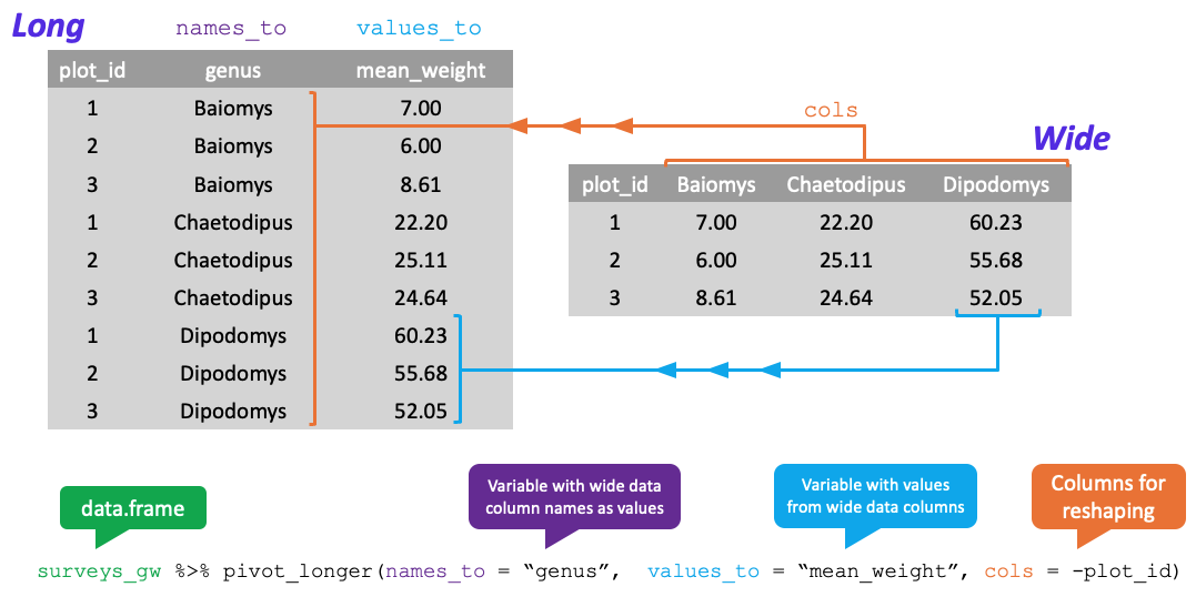
The core syntax involves three main arguments:

cols: The columns you want to pivot or "gather up." These are the columns whose names are actually values of a variable.
names_to: A string specifying the name of the new column that will store the names of the original wide columns. For example, "visit".
values_to: A string specifying the name of the new column that will store the cell values from the original wide columns. For example, "blood_pressure".

This diagram provides a clear visual of the transformation.

This image illustrates the transformation from a wide to a long format. The columns `Baiomys`, `Chaetodipus`, and `Dipodomys` are gathered into a new `genus` column, and their corresponding cell values are placed in a new `mean_weight` column.

The "R for Data Science" e-book offers a fantastic, in-depth explanation of this process.

5 Data tidying

This chapter provides the canonical explanation of pivot_longer(), starting with the "why" and moving into detailed examples of the "how."

First, read Section 5.3.1, "Data in column names". This example, using music chart data, is a classic demonstration of pivot_longer(). Pay close attention to how starts_with("wk") is used to select the columns to pivot and how the names_to and values_to arguments create the new week and rank columns. Also, note the useful values_drop_na = TRUE argument. Next, study Section 5.3.2, "How does pivoting work?". The simple blood pressure example and the accompanying diagrams offer a clear mental model for how the function deconstructs the wide data and reassembles it in long format.

To see this in action, the "Equitable Equations" video provides a practical walkthrough with a dataset very similar to what you might encounter in your own research.

Tidying Data in R with pivot_longer()

This video walks through a complete example of tidying data with pivot_longer(), from identifying the problem to implementing the solution and cleaning the result.

Watch the introduction from the beginning to understand the sample body_temps dataset, a typical "wide" format with repeated measures. Follow the main demonstration from basic syntax, where the presenter uses pivot_longer() with its core arguments. Observe how starts_with() can make column selection easier in the clip from syntax options. This is the same Tidyselect helper you've used with dplyr::select(). Finally, see how to handle missing values that can arise from pivoting in the section on dropping NAs.

As you can see, pivot_longer() is not just a function; it's a way of thinking about your data's structure and how to make it conform to a more powerful, analyzable format.

3. Let's Practice

Now it's time to apply this to a clinical example. Let's imagine we have data from a small trial tracking a biomarker at different time points for several patients.

Open a new R script in your RStudio project and name it 15-pivot-longer.R.

Create the dataset. First, load the tidyverse and create the following "wide" data frame. This tibble shows five patients, the treatment group they belong to, and their biomarker levels measured at baseline, 6 months, and 12 months.
```
library(tidyverse)

patient_biomarkers_wide <- tibble::tribble(
  ~patient_id, ~treatment_group, ~biomarker_baseline, ~biomarker_6mo, ~biomarker_12mo,
  "ID01", "Drug A", 25.4, 22.1, 19.8,
  "ID02", "Placebo", 30.1, 31.0, 30.5,
  "ID03", "Drug A", 28.9, 25.6, NA,
  "ID04", "Drug B", 22.5, 20.1, 18.9,
  "ID05", "Placebo", 27.8, 27.5, 28.1
)
```
Notice that the biomarker measurements are spread across three columns. This is not tidy. To analyze the change over time, we need to reshape it.
Your Task: Create a new data frame called patient_biomarkers_long.
- Start with the patient_biomarkers_wide data frame.
- Pipe it into pivot_longer().
- For the cols argument, select all columns that start with "biomarker_".
- For the names_to argument, create a new column named "visit".
- For the values_to argument, create a new column named "biomarker_level".
- After the pivot_longer() call, add another pipe to drop_na(biomarker_level) to remove the row for the patient with a missing 12-month value.
- Finally, print your new patient_biomarkers_long data frame to the console to inspect it.

Click here to see the solution

patient_biomarkers_long <- patient_biomarkers_wide %>%
  pivot_longer(
    cols = starts_with("biomarker_"),
    names_to = "visit",
    values_to = "biomarker_level"
  ) %>%
  drop_na(biomarker_level)




# Print the result
print(patient_biomarkers_long)

Your resulting tibble should have 14 rows and 4 columns: patient_id, treatment_group, visit, and biomarker_level. Notice how much easier it would be now to plot biomarker_level against visit, perhaps with different colors for each treatment_group.

4. Advanced Reshaping: Splitting Column Names

Sometimes, column names in wide data contain multiple pieces of information. For example, visit1_biomarker and visit1_bp encode both the visit number and the measurement type. pivot_longer() has a clever way to handle this by splitting the names into multiple new columns during the pivot.

The "Epi R Handbook" provides an excellent example from epidemiology where column names contain both an observation number and a data type (obs1_date, obs1_status).

12 Pivoting data – The Epidemiologist R Handbook

This section tackles a more complex, but very realistic, pivoting scenario. It shows how to prevent mixing data types (like dates and characters) into a single column.

Read the section on "Pivoting data of multiple classes". Focus on how names_to = c("observation", ".value") and names_sep = "_" are used. The special ".value" tells pivot_longer that part of the original column name should become the new column header for the values, effectively creating multiple value columns (date and status in their example) and preserving their data types.

This is an advanced technique, but it's incredibly powerful for tidying complex datasets that are common in research settings. Keeping it in your toolkit will save you a lot of manual cleaning steps down the line.

Conclusion

You have now learned one of the most transformative skills in data wrangling: reshaping data from wide to long format. This process is fundamental to creating tidy, analyzable datasets and unlocks the ability to work effectively with dplyr and ggplot2. While it might seem complex at first, the underlying principle is simple: get your data into a structure where each column is a variable and each row is an observation.

Key Takeaways:

Tidy Data: The goal of data wrangling is often to create tidy data, where each variable is a column, each observation is a row, and each value is a cell.
Wide vs. Long: Wide data spreads a single observation across multiple columns. Long data gives each observation its own row.
pivot_longer(): This is the primary function for converting data from wide to long format.
Core Arguments: The function is driven by cols (which columns to reshape), names_to (the name of the new key column), and values_to (the name of the new value column).
Advanced Pivoting: You can handle complex cases, such as splitting a single column name into multiple new variables, using arguments like names_sep and the special ".value" sentinel.

Preview of the Next Lesson:
Having mastered pivot_longer(), the natural next step is to learn its counterpart. In the next lesson, we will explore tidyr::pivot_wider(), which does the exact opposite: it takes a long, tidy dataset and makes it wider. This is useful for creating summary tables for reports or for exporting data to systems that require a wide format.

Recommended resources