Introduction
In our last lesson, you mastered left_join(), a powerful tool for combining datasets—a frequent task in clinical research where patient data might be spread across multiple files. As you saw in our practice exercise, joining data often reveals gaps, resulting in missing values, which R represents as NA. These NAs are not just empty cells; they are a critical feature of real-world data that can break analyses and lead to incorrect conclusions if not handled thoughtfully.
This lesson directly addresses that challenge. We will explore the nature of missing data and learn a precise, "surgical" method for handling it. You will learn how to use the function tidyr::drop_na() to selectively remove rows that have missing values in columns essential for your analysis, while preserving as much valuable data as possible. This is a fundamental step in data cleaning and preparation, moving you closer to producing reliable and reproducible research.
1. The Challenge of Missing Data
In an ideal world, every observation in your dataset would be complete. In reality, especially with clinical data, this is rarely the case. A patient might miss a follow-up appointment, a lab sample might be unusable, or a survey question might be skipped. The result is a dataset peppered with NA values.
Before we learn how to remove them, it's crucial to understand why they need our attention. Many R functions, particularly those used for statistical summaries and modeling, are designed to fail when they encounter NA. For example, trying to calculate the mean() of a vector containing an NA will simply return NA, because R cannot mathematically determine the correct average.
Visualizing the pattern of missingness can be very insightful. The plot below shows a common scenario in a dataset where some variables are nearly complete, while others have significant gaps.

Seeing a plot like this raises a critical question: what should we do? One naive approach is "listwise deletion"—deleting any row that contains any missing value. However, in a dataset like the one shown above, this could mean discarding a huge portion of your data, potentially throwing away valid information from other columns and introducing bias into your analysis. This is why a more targeted approach is necessary.
The video "Handling Missing Data" from R Programming 101 has an excellent segment that explains the importance of this targeted, "surgical" approach.
Handling Missing Data and Missing Values in R Programming | NA Values, Imputation, naniar Package
This video clearly illustrates why indiscriminately deleting all rows with missing values is a bad strategy and introduces the concept of surgically removing only the rows that are problematic for a specific analysis.
Please watch the section from "how to deal with missing values". Pay close attention to the example using the starwars data. The speaker explains why you would lose important data on C-3PO and R2-D2 if you deleted rows based on missing hair_color when your analysis is focused on mass and height.
As the video argues, the best strategy is often to remove only those rows that are missing data in the specific variables you need for your current analysis. This is precisely what tidyr::drop_na() allows us to do.
2. Using tidyr::drop_na() for Targeted Removal
The tidyr package, part of the tidyverse, provides drop_na() as a flexible and readable function for handling missing values. It's a significant improvement over base R's na.omit(), which performs the aggressive listwise deletion we want to avoid.
The R-Bloggers article, "How to Use drop_na," provides a comprehensive guide to its syntax and usage.
How to Use drop_na to Drop Rows with Missing Values in R: A Complete Guide | R-bloggers
This guide walks through the function's capabilities, from basic to advanced use, and highlights important best practices.
In the "Getting Started with drop_na" section, review the "Basic Usage" example. This shows how drop_na() with no arguments removes any row with at least one NA. Next, focus on the "Advanced Usage of drop_na" section, specifically the part on "Targeting Specific Columns". This is the core of today's lesson. Notice how you can provide column names to the function. A row is only dropped if it has an NA in one of the specified columns. Finally, read the "Common Pitfalls" section, particularly the point about "Dropping too much data". This reinforces the importance of being selective and always checking how much data you've lost after cleaning.
To summarize the key syntax:
data %>% drop_na(): Removes all rows containing anNAin any column. Use with caution.data %>% drop_na(column_a): Removes rows only if they have anNAincolumn_a.data %>% drop_na(column_a, column_b): Removes rows if they have anNAincolumn_aORcolumn_b.
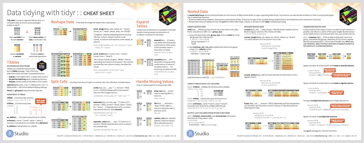
As a quick reference, the tidyr cheat sheet highlights drop_na() and other related functions for handling missing values.
3. Let's Practice
Let's return to our clinical-trial-practice project. In the last lesson, we created the full_clinical_data data frame by joining our patient data with a key for Gleason risk categories. This process introduced NAs into the risk_category column for patients whose sGS (Surgical Gleason Score) was not in our key.
Now, imagine we want to build a model or create a plot examining the relationship between PSADensity (PSA Density) and the risk_category. For this specific analysis, any patient missing a value for either of these two variables is unusable. We need to create a clean dataset for this task.
Open your RStudio project and create a new R script named 14-missing-values.R.
-
Load packages and recreate the joined data frame. This code is the same as the end of our last lesson.
library(tidyverse) library(medicaldata) # Recreate the data from the previous lesson blood_storage_modified <- blood_storage %>% mutate( PSADensity = PreopPSA / PVol, AgeCat = case_when( Age < 70 ~ "Under 70", Age >= 70 ~ "70 and over" ) ) gleason_risk_key <- tibble::tribble( ~score, ~risk_category, 6, "Low Grade", 7, "Intermediate Grade", 8, "High Grade", 9, "High Grade", 10, "Very High Grade" ) full_clinical_data <- blood_storage_modified %>% left_join(gleason_risk_key, by = c("sGS" = "score")) -
Inspect the missing data. Before we remove anything, let's confirm where the
NAs are. Thesummary()function gives a quick overview.summary(full_clinical_data)Look at the counts of
NA'sat the bottom of the output for columns likePSADensityandrisk_category. ThesGSscore of5andNAdid not have a match ingleason_risk_key, creatingNAs inrisk_category. There might also be pre-existingNAs inPSADensity. -
Your Task: Create a new data frame called
analysis_datathat is ready for our hypothetical analysis.- Start with the
full_clinical_dataframe. - Use a pipe (
%>%) to pass it todrop_na(). - Tell
drop_na()to only remove rows that have missing values in thePSADensitycolumn or therisk_categorycolumn. - After creating
analysis_data, print the number of rows in both the original and new data frames to see how many observations were removed. You can get the number of rows withnrow().
- Start with the
Click here to see the solution
# Create the clean data frame for analysis
analysis_data <- full_clinical_data %>%
  drop_na(PSADensity, risk_category)


# Compare the number of rows
cat("Original number of rows:", nrow(full_clinical_data), "\n")
cat("Number of rows after dropping NAs:", nrow(analysis_data), "\n")
cat("Number of rows removed:", nrow(full_clinical_data) - nrow(analysis_data), "\n")


# You can also run summary() on the new data frame to confirm
# that there are 0 NA's in PSADensity and risk_category.
summary(analysis_data)
This exercise demonstrates the core principle of targeted data cleaning. We have prepared a dataset for a specific task without unnecessarily discarding data that might be useful for other analyses (e.g., an analysis that only involves Age and PVol, which might not have been missing in the rows we dropped).
Conclusion
In this lesson, you've moved from simply identifying NAs to strategically handling them. This is a vital step in the data wrangling process, ensuring your subsequent analyses are both technically possible and scientifically valid. You now understand that the goal isn't just to eliminate NAs, but to do so with clear intent, preserving the integrity and size of your dataset as much as possible.
Key Takeaways:
- Missing values (
NA) are common in real-world data and can cause errors in statistical functions and models. - Aggressively removing every row with any missing value (listwise deletion) is often a poor strategy that leads to unnecessary data loss.
tidyr::drop_na()is thetidyversetool for removing rows with missing values.- The most powerful feature of
drop_na()is its ability to target specific columns:data %>% drop_na(critical_col1, critical_col2). This removes only the rows that are unusable for a particular analysis. - Always assess the extent of missing data before and after removal to understand the impact on your dataset.
Preview of the Next Lesson:
So far, we have focused on manipulating the contents and completeness of our data frame's rows and columns. However, sometimes the very structure of the data needs to be changed for effective analysis or visualization. In our next lesson, we will dive into data reshaping with tidyr::pivot_longer(), learning how to transform data from a "wide" format (many columns) to a "long" format (many rows), a foundational technique for advanced analysis in R.