Transforming Data with `mutate` and `map`

1. Applying Non-Vectorized Functions with mutate

You've used mutate() to create new columns with functions that work naturally on vectors, like new_col = old_col * 2 or new_col = log(old_col). But what happens when the function you want to use is designed to work on a single value (a "scalar"), not a whole vector?

Many base R functions, or custom functions using simple if/else statements, are scalar. They expect a single input and return a single output. If you try to use them directly in mutate() on a whole column, R will often throw a warning and produce an incorrect result, because the function only processes the first element of the column.

This is a common hurdle, but purrr provides the perfect solution. Instead of trying to rewrite the function, you can use map() to "tell" mutate() to apply the scalar function to each element of the column individually.

The following reading explains this problem and its solution clearly.

As you can see, the pattern is mutate(new_column = map_variant(column_to_iterate, function_to_apply)). You choose the map variant (_chr, _dbl, etc.) based on the type of output your function produces, just as we did in the last lesson.

Let's say we have our calculate_cv function from before, and we want to apply it not to a column of data, but to a column that contains vectors of data. This brings us to a transformative concept: list-columns.

2. The Power of Nested Data and List-Columns

So far, every column in your data frames has been an "atomic" vector—a simple list of numbers, characters, or logicals. The tidyverse, however, allows for a more complex structure: a list-column. This is a column where each element can be a complex object, such as a vector with a different length, a list, or even an entire data frame.

This structure is exceptionally useful for your goal of analyzing clinical data. Imagine you have data from thousands of patients across different study sites. Instead of keeping it all in one massive table, you can nest it. This creates a data frame with one row per study site, and a list-column named data that contains a smaller data frame with all the patient data for just that site.

Let's see how this works. The following article introduces the concept using the gapminder dataset, nesting it by continent.

Now that you have this powerful way of structuring data, the next logical question is: how do we work with it? How can we calculate a summary statistic for each of the nested data frames? This is where mutate and map come together.

3. Applying Functions to List-Columns

If you have a nested data frame, you can't just call mutate(avg_lifeExp = mean(data$lifeExp)). This will fail because data isn't a single data frame; it's a list of data frames. mutate doesn't know how to operate on it directly.

The solution is to use map() to iterate through the data list-column, apply a function to each data frame inside it, and store the results in a new column.

This diagram illustrates the concept perfectly. We have a list-column (Data), and we use purrr to apply a function to each element, storing the result in a new column.

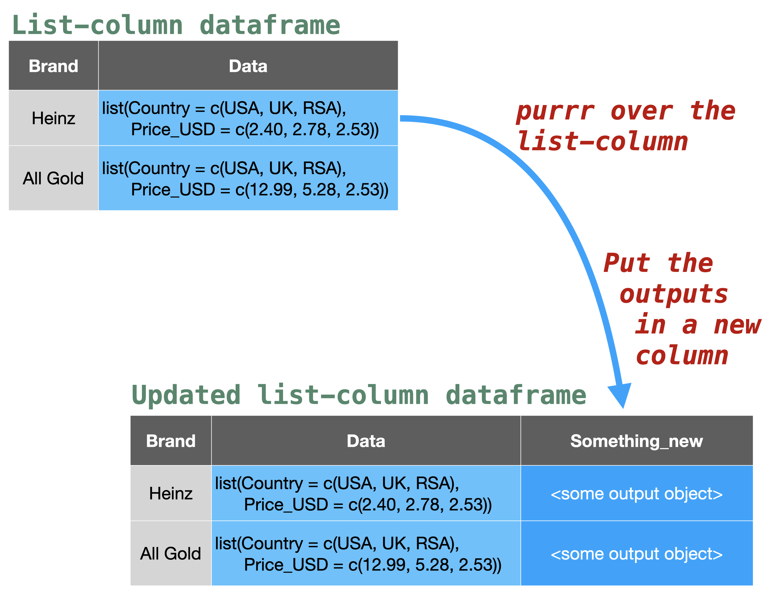
Let's return to the Learn to purrr article to see this in action.

This pattern—group_by(), nest(), mutate() with map()—is one of the most powerful workflows in the tidyverse. It allows you to perform grouped analyses without ever leaving the dplyr pipe, keeping your code organized and readable.

4. A Glimpse of Advanced Analysis

The power of this pattern goes far beyond calculating simple means. You can apply any function, including one that fits a statistical model.

For example, you could fit a separate linear regression model for each continent like this:

library(purrr)
library(dplyr)
library(tidyr)



# (Assuming gapminder_nested is already created)

gapminder_models <- gapminder_nested %>% 
  mutate(model = map(data, ~lm(lifeExp ~ year, data = .x)))

print(gapminder_models)

This code adds a new list-column named model, where each element is a complete lm object representing the model fit for that continent's data. This is a profound concept: you've just performed five separate regression analyses in a single, elegant command.

From here, you could use map2() to iterate over two columns at once—for example, the model column and the data column—to generate predictions for each model.

Finally, looking ahead, you could use a function from the broom package (which you expressed interest in) called broom::tidy() to extract the coefficients from each model into a clean data frame. This is how you scale your statistical analyses efficiently and reliably.

Conclusion

In this lesson, you have connected the functional programming power of purrr with the data manipulation grammar of dplyr. This combination is more than just a convenience; it enables a new paradigm for handling complex, grouped data analysis in a tidy, scalable way.

Key Takeaways:

• mutate + map for Scalar Functions: You can apply functions that only work on single values to an entire column by wrapping the call within a map_*() function inside mutate().
• List-Columns for Nested Data: You can use tidyr::nest() to create list-columns, which store complex objects like data frames inside a column. This is a powerful way to organize data by groups (e.g., by study site, patient cohort, or continent).
• The nest-mutate-map Workflow: The most powerful application of today's lesson is the group_by() %>% nest() %>% mutate(new_col = map(data, ...)) pattern. This allows you to perform complex, group-wise operations—from simple summaries to fitting dozens of statistical models—all within a single, readable pipeline.

Preview of the Next Lesson:
The anonymous functions we used with map() today were relatively simple. As your analyses grow more complex, you'll need to write more sophisticated custom functions. The next lesson will formally cover conditional logic using if and else statements, a fundamental building block for writing functions that can handle different conditions and inputs gracefully.