Hello! In our previous lessons, you've performed a variety of statistical tests, from t-tests and ANOVA to their non-parametric counterparts. You may have noticed a recurring pattern: after running a test, we often used the broom::tidy() function to clean up the output. This was a deliberate preview of a crucial technique in modern R analysis.
Today, we'll dive deep into broom::tidy(). This lesson is dedicated to understanding why this function is so essential and mastering how to use it. We'll explore the problem it solves—the inconsistent and often messy outputs of R's built-in statistical functions—and see how tidy() provides a consistent, predictable, and powerful solution. For your goal of conducting reproducible clinical research, tidying your model outputs is not just a convenience; it's a foundational step for building scalable and reliable analysis pipelines.
By the end of this lesson, you will be able to confidently use broom::tidy() to transform the results of any statistical model into a clean, easy-to-use data frame.
1. The Challenge: Messy Model Outputs
When you run a statistical test in R, the object it returns contains a wealth of information. However, accessing and using that information can be surprisingly difficult. The default print-outs are designed for a human to read in the console, not for a computer to process programmatically.
This video from a presentation by David Robinson, the creator of the broom package, gives a perfect overview of the problem.
Broom: Converting Statistical Models to Tidy Data Frames
Watch the initial segment of "Broom: Converting Statistical Models to Tidy Data Frames."
Focus on the sections that introduce the concept of tidy data (Tidy Data) and then highlight the problems with standard model outputs (Messy Models). As you watch, notice the specific issues he points out: Information is stored in row names, not columns. Column names can be inconsistent and contain spaces or punctuation. Some important values (like a model's F-statistic p-value) are printed but not easily accessible. Every model type has a unique output structure.
These "inconveniences," as he calls them, become significant roadblocks when you need to compare multiple models, plot coefficients, or include results in a report—all common tasks in research.
2. The Solution: The broom Package
The broom package was created to solve this exact problem. It acts as a "sweeper," taking the cluttered output of a statistical model and organizing it into a clean, predictable "tidy" data frame (a tibble).
The package provides three core functions, each serving a different purpose:
tidy(): Summarizes the statistical components of a model. For each parameter (like a predictor in a regression), it provides estimates, p-values, confidence intervals, etc. This is our focus for today.augment(): Adds observation-level data to the original dataset, such as fitted values (predictions) and residuals.glance(): Provides a single-row summary of the entire model's performance, including statistics like R-squared, AIC, or the overall model p-value.
This next segment of the same video introduces these three functions.
Broom: Converting Statistical Models to Tidy Data Frames
Continue watching the "Broom" video.
Pay close attention to the introduction of the tidy() function (introducing tidy) and the overview of the three main broom functions: tidy(), augment(), and glance() (three methods). This will give you a clear mental model of how broom organizes model information.
3. Using broom::tidy() in Practice
The beauty of broom is its consistency. Regardless of the model you fit, you can almost always pipe the result directly into tidy(). Let's see this in action with some of the models you've already learned.
T-Test
Remember running a t-test. The standard output is informative but clunky. With broom, it becomes a neat, single-row tibble.
Chapter 8 Part 6: Simple Statistics with broom - Ready for R
This chapter from "Ready for R" provides clear, hands-on examples of using broom.
Focus on section 8.5.4 t-test. Notice how the code t.test(...) %>% tidy() transforms the multi-line console output into a structured tibble with clearly named columns. You can skim the setup and data exploration parts.
This is the basic workflow:
# Example of a paired t-test from the resource
# t.test(data$var1, data$var2, paired = TRUE) %>%
#   broom::tidy()


## # A tibble: 1 x 8
##   estimate statistic p.value parameter conf.low conf.high method      alternative
##      <dbl>     <dbl>   <dbl>     <dbl>    <dbl>     <dbl> <chr>       <chr>
## 1   -0.207     -1.78  0.0774        97   -0.438    0.0232 Paired t-t… two.sided
Linear Regression (lm())
The benefit becomes even more apparent with regression models, which have multiple coefficients. The standard summary(lm_model) output is difficult to work with. tidy() converts it into a data frame where each row represents one coefficient from your model.
Chapter 8 Part 6: Simple Statistics with broom - Ready for R
Now, read the section 8.7 Let’s build a simple linear model in the same resource.
Follow the example where a linear model is created with lm(dxa ~ st, data=body_comp). Contrast the complex standard summary (which isn't even shown) with the clean output from piping the model into tidy().
Here's the code pattern:
# lm(outcome ~ predictor1 + predictor2, data = my_data) %>%
#  broom::tidy()


## # A tibble: 3 x 5
##   term        estimate std.error statistic  p.value
##   <chr>          <dbl>     <dbl>     <dbl>    <dbl>
## 1 (Intercept)   0.0646    0.224      0.288 7.74e- 1
## 2 st            0.888     0.0362    24.5   6.93e-43
## 3 gender0       0.577     0.222      2.60  1.09e- 2
This principle extends to virtually all the models you've seen, including ANOVA (aov()), chi-square tests (chisq.test()), and the non-parametric tests from our last lesson (wilcox.test(), kruskal.test()). The command is always the same: ... %>% broom::tidy().
4. Understanding the Tidy Output
The tidy() function consistently produces a data frame with standardized column names. While the exact columns may vary slightly between model types, you will almost always see these key ones:
term: The name of the model component being described. For a regression, this will be the intercept and each predictor variable. For a t-test, there is no term.estimate: The calculated value for the term. For a regression coefficient, this is its estimated value. For a t-test, it might be the difference in means.std.error: The standard error of the estimate, which measures its uncertainty.statistic: The test statistic (e.g., a t-value or z-score) used to calculate the p-value.p.value: The p-value for that specific term, testing its significance.conf.lowandconf.high: The lower and upper bounds of the confidence interval for the estimate.
The resource below, from a book on reproducible medical research, provides another excellent walkthrough and explicitly discusses how to interpret these tidy outputs.
Chapter 32 Linear Regression and Broom for Tidying Models | Reproducible Medical Research with R
This chapter reinforces the use of broom in a medical research context.
First, read the introductory text and the example in section 32.1.1, which shows lm() being piped into broom::tidy(). Then, jump to section 32.2.0.3 Interpreting the Model Estimates. This section provides a clear explanation of what the term and estimate columns represent in the context of a linear model.
While we've briefly defined these columns, our entire next lesson will be dedicated to interpreting them in depth for different models, turning this tidy data into meaningful conclusions for your research.
5. The Power of a Tidy Workflow
Why do we care so much about this tidy format? Because once your model results are in a data frame, you can use all the dplyr and ggplot2 skills you've been learning to analyze and present them.
1. Easy Visualization: You can pipe a tidied model directly into ggplot2 to create coefficient plots. This is a standard and highly effective way to visualize model results in publications.
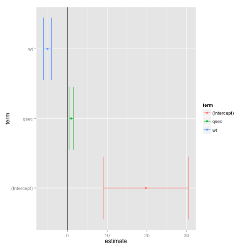
2. Comparing and Combining Models: In clinical research, you often need to run the same model on different subgroups of patients (e.g., by age group or disease severity) or compare different models. Because tidy() produces a standard data frame, you can easily run multiple models, tidy each one, and then stack the results into a single data frame for comparison or plotting.
This final clip from the broom video brilliantly illustrates this power.
Broom: Converting Statistical Models to Tidy Data Frames
Watch the last major section of the video.
First, see how tidied data frames are fed directly into ggplot2 to create plots like the coefficient plot and survival curves (visualizing tidy models). Then, watch the section on how this enables the combination and comparison of many models at once (combining models), a technique incredibly useful for subgroup analyses or bootstrapping.
Conclusion
You have now formally added broom::tidy() to your R toolkit. You understand the fundamental problem of inconsistent model outputs and how broom provides an elegant, tidy solution. This function is a bridge that connects the world of statistical modeling with the world of data manipulation and visualization in the Tidyverse.
Key Takeaways:
- Standard R model objects are often "messy," with inconsistent structures that make them hard to use programmatically.
- The
broom::tidy()function converts messy model outputs into clean, predictable data frames (tibbles). - The workflow is simple and consistent: run your model, then pipe the result into
tidy(). - A tidied data frame has standard column names like
term,estimate, andp.value, which are easy to work with. - Once model results are tidy, you can easily visualize them with
ggplot2or combine results from multiple models for advanced comparisons.
Preview of the Next Lesson:
Now that you know how to get your results into a tidy format, the next step is to master their interpretation. In our next lesson, we will focus on the key columns produced by broom::tidy()—estimate, p.value, conf.low, and conf.high—and learn how to interpret their meaning across different types of statistical models.