Interpreting broom::tidy() Output

From Numbers to Narrative: Interpreting Tidy Model Outputs

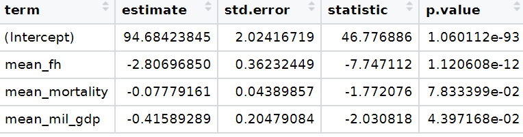
The output of broom::tidy() provides a concise summary of a statistical model's components. Let's break down the most important columns, using examples you've seen before. The result is always a tibble, like the one shown below, where each row corresponds to a specific parameter or term in your model.

1. The term and estimate Columns: Quantifying Effects

The term column identifies the specific part of the model being described in that row. The estimate column provides the point estimate—the model's "best guess" for the value of that term based on your data. Its meaning, however, depends entirely on the model and the term.

In a T-Test

For a two-sample t-test, there is typically only one primary estimate: the difference in the means between the two groups.

In the example from the reading, the output looks like this:

## # A tibble: 1 x 8
##   estimate statistic p.value parameter conf.low conf.high method      alternative
##      <dbl>     <dbl>   <dbl>     <dbl>    <dbl>     <dbl> <chr>       <chr>
## 1   -0.207     -1.78  0.0774        97   -0.438    0.0232 Paired t-t… two.sided

Here, the estimate of -0.207 represents the estimated mean difference between the dxa and st measurements. A negative value indicates that the mean of the first variable (dxa) is 0.207 units lower than the mean of the second variable (st). In a research paper, you might report this as: "The skin-fold thickness method overestimated body fat by an average of 0.207 percentage points compared to the DXA method."

In a Linear Regression (lm())

In a linear regression, broom::tidy() provides a row for each coefficient in the model.

• (Intercept): The estimate for this term is the predicted value of your outcome variable when all predictor variables in the model are equal to zero.
• Predictor Variables: The estimate for a predictor variable (e.g., mean_fh in the image above) is its slope. It represents the average change in the outcome variable associated with a one-unit increase in that predictor, holding all other variables in the model constant.

Let's examine this in a practical context.

The output shows:

## # A tibble: 2 x 5
##   term        estimate std.error statistic  p.value
##   <chr>          <dbl>     <dbl>     <dbl>    <dbl>
## 1 (Intercept)    0.275     0.215      1.28 2.05e- 1
## 2 st             0.903     0.0367    24.6  3.17e-43

• The estimate for (Intercept) is 0.275. This means that if a child had a skin-fold thickness (st) measurement of 0, their predicted dxa body fat would be 0.275. In many clinical contexts, a value of 0 for a predictor is not biologically possible or meaningful, so the intercept is often just a mathematical component of the model rather than a point of direct interpretation.
• The estimate for st is 0.903. This is the slope. It means that for every one-unit increase in the st measurement, the predicted dxa measurement increases by 0.903 units.

2. The p.value Column: Assessing Statistical Significance

The p-value tests a specific null hypothesis for each term. In most models, the null hypothesis is that the true value of the estimate is zero.

• A small p-value (typically < 0.05) provides evidence against the null hypothesis. It suggests that the effect or relationship you observed in your sample is unlikely to be due to random chance alone. You would conclude the term is "statistically significant."
• A large p-value (typically >= 0.05) means you do not have sufficient evidence to reject the null hypothesis. The observed effect could plausibly be due to random variation. You would conclude the term is "not statistically significant."

Looking back at our lm() example, the p-value for the st term is 3.17e-43, which is an extremely small number. This allows us to confidently reject the null hypothesis that the true relationship between st and dxa is zero. We can conclude there is a highly significant statistical relationship.

3. conf.low and conf.high: The Range of Plausible Effects

While the estimate gives a single "best guess," the confidence interval (CI), defined by conf.low and conf.high, provides a range of plausible values for the true effect in the population. By default, broom::tidy() calculates a 95% confidence interval. This means if you were to repeat your study 100 times, you'd expect the true population value of the parameter to be contained within the calculated interval in about 95 of those studies.

To get the confidence intervals, you must add the argument conf.int = TRUE to the tidy() function.

# lm(dxa ~ st, data = body_comp) %>%
#  broom::tidy(conf.int = TRUE)




## # A tibble: 2 x 7
##   term        estimate std.error statistic  p.value conf.low conf.high
##   <chr>          <dbl>     <dbl>     <dbl>    <dbl>    <dbl>     <dbl>
## 1 (Intercept)    0.275    0.215       1.28 2.05e- 1   -0.153     0.703
## 2 st             0.903    0.0367     24.6  3.17e-43    0.830     0.976

Here, the 95% CI for the st term is [0.830, 0.976]. We can state that we are 95% confident that the true increase in dxa for every one-unit increase in st is somewhere between 0.830 and 0.976.

The Connection Between CIs and P-values

The confidence interval provides a direct link to the p-value. For a 95% CI:

If the interval does not contain zero, the p-value will be less than 0.05.
If the interval does contain zero, the p-value will be greater than or equal to 0.05.

Notice for the st term, the interval [0.830, 0.976] is entirely positive and does not cross zero, which aligns with its tiny p-value. For the (Intercept) term, the interval [-0.153, 0.703] does cross zero, which aligns with its non-significant p-value of 0.205.

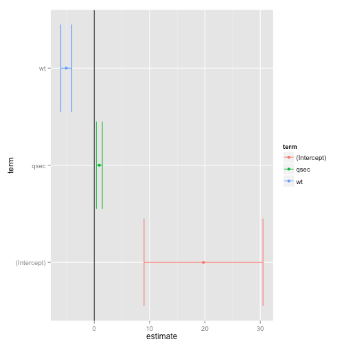
This is why coefficient plots are so powerful in research papers. They visualize both the estimate (the point) and the confidence interval (the whiskers). You can immediately see which effects are statistically significant by checking if their CI whiskers cross the zero line.

4. Case Study: Interpreting a Multiple Regression Model

Let's put this all together by interpreting a more complex model from a medical context. This example models the factors influencing post-operative throat pain.

The tidied output for the full model is:

## # A tibble: 6 × 5
##   term                estimate std.error statistic p.value
##   <chr>                  <dbl>     <dbl>     <dbl>   <dbl>
## 1 (Intercept)            0.376    0.365      1.03  0.304
## 2 intraOp_surgerySize    0.316    0.143      2.21  0.0283
## 3 treat                 -0.690    0.154     -4.48  0.0000117
## 4 preOp_pain             1.96     0.835      2.35  0.0197
## 5 preOp_gender          -0.265    0.160     -1.65  0.100
## 6 preOp_smoking          0.0652   0.0956     0.682 0.496

Here is how you would interpret these results for a publication:

• Treatment (treat): The licorice gargle treatment had a statistically significant effect on reducing post-operative throat pain. On average, patients in the treatment group had a pain score that was 0.690 points lower than patients in the control group, holding all other variables constant (estimate = -0.690, p.value < 0.001).
• Surgery Size (intraOp_surgerySize): The size of the surgery was significantly associated with throat pain. For each one-unit increase in surgery size, the average pain score increased by 0.316 points (estimate = 0.316, p.value = 0.028).
• Pre-operative Pain (preOp_pain): Patients who reported pre-operative pain had significantly higher post-operative pain scores, with an average increase of 1.96 points compared to those without pre-operative pain (estimate = 1.96, p.value = 0.020).
• Gender (preOp_gender) and Smoking (preOp_smoking): Neither gender nor smoking status were found to be statistically significant predictors of post-operative throat pain in this model (p-values of 0.100 and 0.496, respectively).

This narrative translates the numeric output into a clear, concise summary of the study's findings—the ultimate goal of your analysis.

Conclusion

In this lesson, you moved from simply generating tidy output to interpreting it with scientific rigor. You now understand how to dissect the output of broom::tidy() to tell a story with your data.

Key Takeaways:

• The estimate column provides the point estimate of an effect, which could be a difference in means (t-test) or a slope coefficient (linear regression).
• The p.value tests the null hypothesis that the true estimate is zero, allowing you to assess statistical significance.
• The conf.low and conf.high columns define the 95% confidence interval, a range of plausible values for the true population effect.
• A confidence interval that does not contain zero corresponds to a p-value less than 0.05, providing a quick visual check for significance.
• Interpreting these columns together allows you to report on the direction, magnitude, and statistical significance of effects, which is the core of reporting quantitative research.

Preview of the Next Lesson:
So far, you've learned to test hypotheses and interpret the tidy results. In the next module, "Regression Modeling," we will take a step back and focus on the models themselves. You will learn how to properly fit a simple linear regression model using lm(), and crucially, how to assess the underlying assumptions that must be met for your interpretations to be valid.