Welcome back! In our last two lessons, you learned how to build a simple linear regression model and, just as importantly, how to rigorously diagnose its underlying assumptions. You now have a solid foundation for understanding the relationship between a single predictor and a continuous outcome.
Today, we take a significant step forward into a more powerful and realistic analytical technique: multiple linear regression. In most research scenarios, especially in clinical studies, an outcome is influenced by more than one factor. Multiple regression allows you to model this complexity, assessing the unique contribution of each predictor while statistically "controlling for" the effects of the others. This lesson will equip you with the skills to fit these models in R and, crucially, to interpret their results with the nuance required for high-quality research.
From Simple to Multiple Regression: The Power of Adjustment
Why can't we just run separate simple regressions for each predictor? The reason is that predictors are often related to each other. Multiple regression's greatest strength is its ability to disentangle these relationships. It isolates the association between one predictor and the outcome, after accounting for the influence of all other predictors in the model. This concept is often described as "adjusting for" or "controlling for" other variables.
To understand this core idea, let's explore an excellent blog post from "Stats and R" that illustrates this concept.
Multiple linear regression made simple
This article provides a clear, practical introduction to the principles of multiple linear regression. We'll start by focusing on the "why" and the basic equation.
First, read the section Principle. Pay close attention to the example where the estimated coefficient for wt (weight) changes when hp (horsepower) and disp (displacement) are added to the model. This demonstrates the concept of "adjustment." Then, read the brief Equation section to see how the mathematical formula is extended from simple regression.
The key takeaway is that the coefficient for a predictor in a multiple regression model represents its unique contribution. It's the effect of that predictor on the outcome, holding all other variables in the model constant.
Fitting a Multiple Regression Model in R
The good news is that fitting a multiple regression model in R is a straightforward extension of what you already know. You simply add more predictors to the formula using the + operator.
Let's watch a quick demonstration of the syntax.
Multiple linear regression in R
This video from the Equitable Equations channel shows the basic R syntax for building a multiple regression model.
Watch the short segment from the beginning of the "The Model" section. Notice how the formula y ~ x1 + x2 is a simple and intuitive extension of the lm() function you've used before.
As you can see, the code is simple. The real skill lies in interpreting the output.
Interpreting the Model Output
The summary() output of a multiple regression model contains a wealth of information. Let's break down how to interpret it correctly, which is vital for communicating your research findings.
Interpreting Coefficients: "All Else Being Equal"
The most critical skill is interpreting the coefficients table. Each predictor gets its own row with an Estimate, Std. Error, t value, and p.value. The interpretation of the Estimate must always include the "ceteris paribus" (all other things being equal) condition.
The "Stats and R" article provides an excellent guide with template sentences for interpreting both quantitative and qualitative predictors. Mastering this phrasing is key to precise statistical communication.
Multiple linear regression made simple
This next section is the most important part of today's lesson. It provides clear templates for correctly interpreting the coefficients from a multiple regression model, a skill central to your goal of producing publication-quality analyses.
Please study the entire section Interpretations of coefficients. For quantitative variables (like wt), focus on the phrasing: "for an increase of one unit in [predictor], the [outcome] changes, on average, by [estimate], for a constant level of [other predictors]." For qualitative variables (like vs, engine shape), notice how the interpretation is about comparing one level to the reference level: "...increases by, on average, [estimate] when [level] compared to [reference level], for a constant [other predictor]."
This verbal walkthrough from MarinStatsLectures reinforces these concepts and also explains the overall model statistics.
Multiple Linear Regression in R | R Tutorial 5.3 | MarinStatsLectures
This tutorial provides an excellent verbal explanation of the summary() output, tying all the pieces together.
Watch the segment from the summary walkthrough. Listen carefully to how the speaker interprets the slope for age as "adjusting or controlling for height." This is the language you should use. Also, pay attention to the explanation of the overall model F-statistic and R-squared. Then, continue watching from obtaining confidence intervals to see how to use confint() on a multiple regression model.
Understanding the Overall Model
Beyond individual coefficients, you need to assess the model as a whole.
- F-statistic and p-value: This tests the null hypothesis that all your predictor coefficients are simultaneously equal to zero. A small p-value (< 0.05) suggests that your model, as a whole, is better at predicting the outcome than a model with no predictors (i.e., just the intercept).
- Multiple R-squared & Adjusted R-squared: As in simple regression,
R-squaredis the proportion of variance in the outcome explained by your predictors. However,R-squaredalways increases when you add more variables, even useless ones. Therefore, in multiple regression, we prefer the Adjusted R-squared. It penalizes the R-squared value for each extra predictor added, providing a more honest measure of model fit. A higher adjusted R-squared generally indicates a better model.
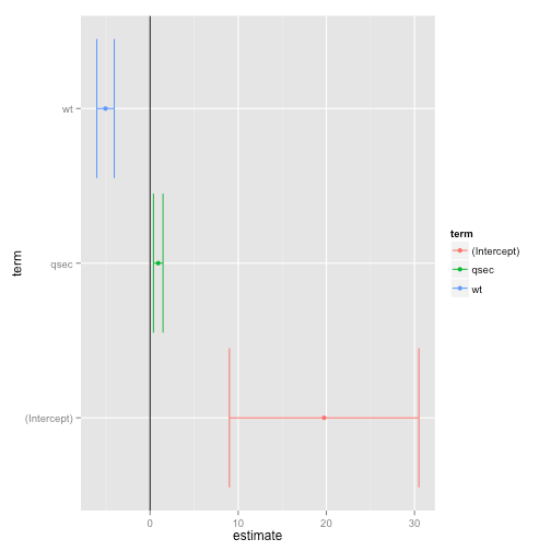
A coefficient plot can be a great way to visualize the estimates and their uncertainty (confidence intervals) for multiple predictors at once.
A New Assumption: Checking for Multicollinearity
When you have multiple predictors, you must check for a new issue: multicollinearity. This occurs when two or more predictor variables in the model are highly correlated with each other.
Why is this a problem? If two predictors are highly correlated, the model has trouble distinguishing their individual effects on the outcome. This can lead to:
- Unstable and unreliable coefficient estimates. A small change in the data could cause large swings in the estimated coefficients.
- Inflated standard errors, which can make a significant predictor appear non-significant.
The most common way to diagnose multicollinearity is by calculating the Variance Inflation Factor (VIF) for each predictor.
Chapter 9 Multiple regression | Statistics in Natural Resources: Applications with R
This resource from "Statistics in Natural Resources" provides a concise explanation of multicollinearity and how to diagnose it using VIF.
Read the section titled 9.3.2 Evaluating multiple linear regression models, starting from the paragraph introducing the concept. Focus on understanding the consequences of multicollinearity and the definition of the Variance Inflation Factor (VIF). A common rule of thumb is that a VIF value greater than 5 or 10 indicates a problematic level of multicollinearity. Note the R code using vif() from the {car} package.
As you may recall from our previous lesson, the performance::check_model() function provides an excellent, all-in-one set of diagnostic plots. Conveniently, it includes a VIF check for multicollinearity, integrating this new step into the workflow you've already learned.
Tidying Your Model with broom
Consistent with your goal of creating clean, reproducible analyses, the broom package works seamlessly with multiple regression models. broom::tidy() will return a clean data frame of your coefficients, while broom::glance() will provide a one-row summary of the overall model statistics.
Chapter 9 Multiple regression | Statistics in Natural Resources: Applications with R
Let's confirm how the broom functions you've used before apply to a multiple regression model object.
In the "Implementation in R" section, review the part that begins here. Observe how tidy(falcon.lm) neatly organizes the coefficient table and glance(falcon.lm) summarizes the model's performance metrics like r.squared and adj.r.squared.
Conclusion
You have now expanded your regression toolkit significantly. Moving from simple to multiple linear regression is a crucial step towards conducting sophisticated data analysis that mirrors the complexity of real-world phenomena, particularly in clinical research where multiple factors are always at play.
Key Takeaways:
- Multiple linear regression models an outcome using several predictors simultaneously, using the syntax
lm(y ~ x1 + x2 + ...). - The interpretation of a coefficient is its effect on the outcome while holding all other predictors in the model constant. This is the core concept of statistical adjustment.
- The Adjusted R-squared is preferred over R-squared for judging model fit, as it accounts for the number of predictors.
- The overall model's significance is assessed with the F-statistic, which tests if at least one predictor is useful.
- A new assumption to check is multicollinearity (highly correlated predictors), which can be diagnosed using the Variance Inflation Factor (VIF).
- The
broompackage'stidy()andglance()functions are essential tools for extracting results from multiple regression models in a reproducible way.
Preview of the Next Lesson:
Our focus so far has been on predicting continuous numerical outcomes. However, many critical questions in clinical research involve binary outcomes: Did a patient respond to treatment (yes/no)? Did the disease recur (yes/no)? Linear regression is not suitable for this. In our next lesson, we will introduce binomial logistic regression, the standard method for modeling these important categorical outcomes.