Following our last session where you learned to fit and interpret a simple linear regression model, we now turn to a critical step in the modeling process: validation. A model is only as good as the assumptions it rests upon. In this lesson, we will address how to rigorously check if your linear regression model is appropriate for your data.
Your goal of producing publication-quality analyses for clinical research demands a deep understanding of model diagnostics. Simply reporting coefficients and p-values is insufficient; you must also demonstrate that the model is statistically valid. Today, you will learn to assess the core assumptions of linear regression by generating and interpreting a standard set of diagnostic plots in R. This skill is fundamental to ensuring the reliability and credibility of your research findings.
The Assumptions of Linear Regression
Before we dive into the plots, let's establish the assumptions we need to check. A helpful mnemonic is LINE:
- Linearity: The relationship between the predictor(s) and the outcome variable must be linear.
- Independence: The errors (residuals) must be independent of each other. This is typically ensured by the study design (e.g., one observation per patient). We won't test this with plots, but it's a crucial conceptual check.
- Normality: The errors should be normally distributed. For larger sample sizes, the central limit theorem provides some robustness to violations of this assumption, but it's always important to check.
- Equal Variance (Homoscedasticity): The variance of the errors should be constant across all levels of the predictor variables. The opposite is heteroscedasticity, where the error variance changes.
An additional check is for influential outliers—single data points that have a disproportionately large effect on the model's results. For your work in clinical research, identifying such a point could mean uncovering a data entry error or a patient with a unique clinical profile that warrants further investigation.
Multiple linear regression made simple
This article from Stats and R provides a clear and concise summary of the key assumptions for linear regression.
Please read the section "Conditions of application". Pay close attention to the list of five conditions and the brief explanation for each. The "LINE" acronym mentioned in the article is a useful way to remember the first four.
Generating and Interpreting Diagnostic Plots
R provides a powerful and simple way to generate the standard set of diagnostic plots for a model object created with lm(). The following video provides a fantastic overview of this process, showing you not only how to create the plots but, more importantly, what to look for.
Checking Linear Regression Assumptions in R | R Tutorial 5.2 | MarinStatsLectures
This tutorial from MarinStatsLectures demonstrates how to generate and interpret the four main diagnostic plots in R, with clear examples of what violations look like.
Please watch the full video from start to finish. As you watch, focus on: The four assumptions: How the video frames the key assumptions. Generating the plots: The use of par(mfrow=c(2,2)) and plot(model) to get all four plots at once. Visualizing violations: The excellent examples showing what heteroscedasticity (a "megaphone shape") and non-linearity (a curved pattern) look like in the plots. The rationale for multiple regression: The final point about why these plots are even more critical when you have multiple predictors.
A Deeper Dive into the Four Key Plots
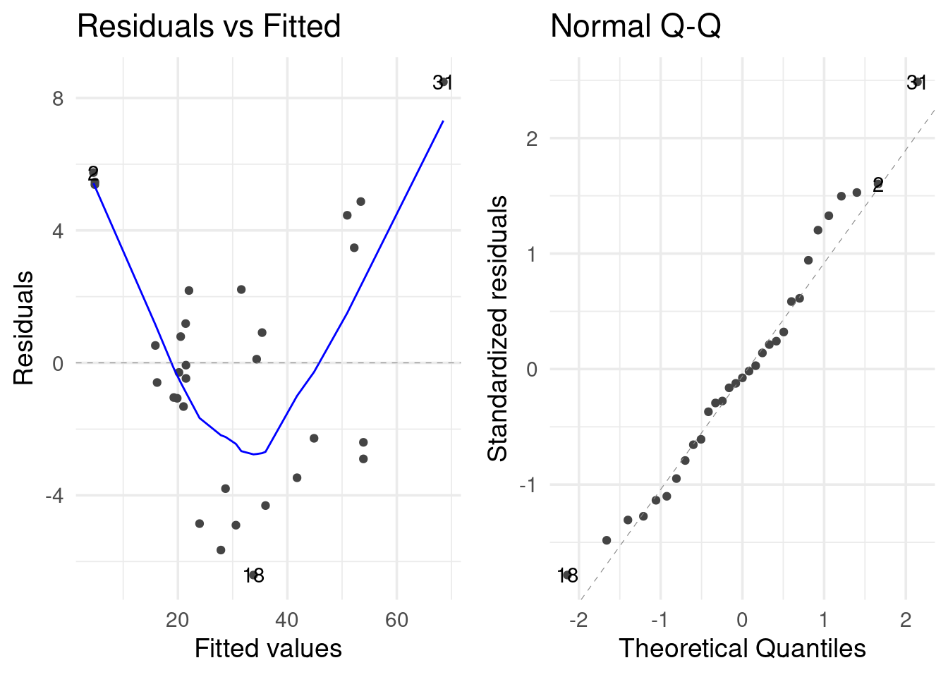
The video gave you a great visual introduction. Now, let's break down each of the four plots you get from plot(model) in more detail. We'll use the plot below, which shows significant violations, to illustrate what to look for.
1. Residuals vs. Fitted Plot
- Purpose: This is your workhorse plot for checking two assumptions at once: Linearity and Homoscedasticity.
- How to Read It:
- The x-axis has the model's fitted (predicted) values.
- The y-axis has the corresponding residuals (the errors).
- For Linearity: The red smoothed line should be roughly horizontal and close to the dashed line at y=0. If it shows a clear curve or pattern (like the U-shape in the example plot), the linearity assumption is violated.
- For Homoscedasticity: The points should form a random "cloud" with a constant vertical spread as you move from left to right. If you see a funnel or megaphone shape where the spread of residuals increases or decreases with the fitted values (as seen in the example), the assumption of equal variance is violated. This is heteroscedasticity.
The video below offers an excellent conceptual walkthrough of this specific plot.
This video from Dataslice gives a detailed explanation of the Residuals vs. Fitted plot, including what heteroscedasticity and non-linear relationships look like.
Watch the segment from Residuals vs. Fitted. The explanation of heteroscedasticity, where the variability of predictions is unequal, is particularly clear and relevant to your work.
2. Normal Q-Q Plot
- Purpose: To check if the residuals follow a Normal Distribution.
- How to Read It:
- This plot compares the quantiles of your standardized residuals (on the y-axis) against the theoretical quantiles of a perfect normal distribution (on the x-axis).
- If the normality assumption holds, the points should fall closely along the dashed diagonal line.
- Violations appear as systematic deviations from the line. In our example plot, the points curve away from the line at both ends, indicating that the tails of our residual distribution are "heavier" than a normal distribution (i.e., we have more extreme outliers than expected).
BIOSTATS 640 2023 R Lesson 08 Regression Diagnostics
This document from a biostatistics course provides a technical summary of checking for normality.
Read the section on "Normality of Residuals". Focus on the "Goal" and "What to watch out for" descriptions for both the histogram and the QQ Plot. Note the author's excellent point about how formal tests like shapiro.test() can be overly sensitive with large sample sizes, making visual inspection of plots even more important.
3. Scale-Location Plot
- Purpose: This is another way to check for Homoscedasticity (equal variance).
- How to Read It:
- It's similar to the Residuals vs. Fitted plot, but the y-axis shows the square root of the standardized residuals. Taking the square root helps to reduce the skew of the residuals, making it easier to see trends in their variance.
- As before, you are looking for a red line that is roughly horizontal and for points that are randomly scattered with no discernible pattern. An upward-sloping line indicates that variance increases with the fitted value.
4. Residuals vs. Leverage Plot
- Purpose: To identify influential data points. An influential point is one that, if removed, would cause a significant change in the model fit. These points are problematic because they have an undue impact on your conclusions.
- How to Read It:
- The y-axis has the standardized residuals (how much of an outlier is the point in the y-direction?).
- The x-axis has the "leverage" (how much of an outlier is the point in the x-direction?).
- Cook's distance, shown by the dashed red lines, combines information about a point's residual and its leverage into a single measure of influence.
- You should be concerned about points that are:
- Far to the right (high leverage).
- Far from the zero line (large residual).
- Most importantly: Points that cross the Cook's distance lines (typically in the top-right or bottom-right corners). These points are flagged as being highly influential.
A Modern, All-in-One Approach
While the base R plot() function is the traditional method, newer packages offer more streamlined and visually appealing ways to conduct diagnostics. The {performance} package is particularly useful for your goal of creating high-quality outputs.
Multiple linear regression made simple
This section of the Stats and R blog post introduces a very convenient function for checking all assumptions at once.
Read the text and examine the plot in the section beginning with this paragraph. The check_model() function from the {performance} package produces a single, well-annotated grid of plots that tests all the assumptions simultaneously. The plot shown in the article is reproduced below for convenience.
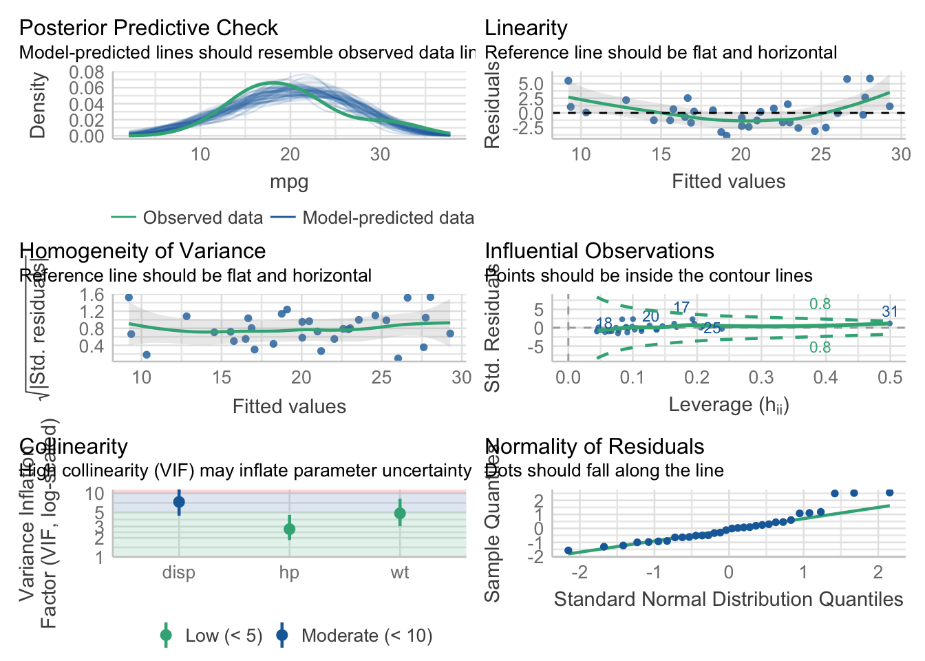
This single command provides clear, ggplot2-based visuals and is an excellent tool for a reproducible analysis report. Notice it also includes a check for Collinearity (or multicollinearity), which we will discuss in the next lesson as it becomes relevant when you have multiple predictors.
Conclusion
You have now learned not only how to fit a linear model but also how to critically evaluate its validity. This diagnostic step is what separates a naive analysis from a rigorous, defensible one. Never trust a model you haven't diagnosed.
Key Takeaways:
- Linear regression relies on the LINE assumptions: Linearity, Independence, Normality, and Equal Variance.
- The base R command
plot(model_object)generates four key diagnostic plots to check these assumptions visually. - Residuals vs. Fitted: Checks for non-linearity (curved red line) and heteroscedasticity (funnel shape).
- Normal Q-Q Plot: Checks for normality of residuals (points should follow the dashed line).
- Scale-Location Plot: Also checks for homoscedasticity.
- Residuals vs. Leverage: Helps identify influential points that fall outside the Cook's distance lines.
- Modern packages like
{performance}offer convenient, all-in-one functions likecheck_model()for streamlined diagnostic reporting.
Preview of the Next Lesson:
With the skills to fit and diagnose a simple linear regression, you are ready to expand your toolkit. In our next lesson, we will move to multiple linear regression, where you will model an outcome using several predictors simultaneously. As the MarinStatsLectures video noted, diagnostics become even more crucial in that context, and we will introduce an additional check for multicollinearity.