Simple Linear Regression with `lm()`

Welcome to the next stage of your journey in statistical analysis. Having mastered the principles of hypothesis testing, including the crucial adjustments for multiple comparisons, you are now ready to move from simply asking if a relationship exists to describing what that relationship looks like. This lesson opens our new module on regression modeling, one of the most powerful and flexible tools in a data analyst's toolkit.

Our goal today is to fit and interpret a simple linear regression model. You will learn to use the lm() function in R to model the relationship between two numeric variables. This involves not only generating the model but also understanding what the output tells us about the strength and nature of the association. This foundational skill is essential for the predictive modeling and causal inference tasks common in clinical research.

From Correlation to Regression

In a previous module, you learned to calculate a correlation coefficient, which measures the strength and direction of a linear relationship. Simple linear regression takes this a step further. Instead of just a single number, it gives us a mathematical equation—a line—that best describes the relationship. This line allows us to quantify the effect of one variable on another and even predict future outcomes.

The equation for a simple linear regression model is:

y^= β_{0} + β_{1} x

Let's break this down:

$y^$ (read "y-hat") is the predicted value of our outcome variable.
$x$ is the value of our predictor variable.
$β_{0}$ (beta-naught) is the intercept: the predicted value of $y$ when $x$ is 0.
$β_{1}$ (beta-one) is the slope: the predicted change in $y$ for a one-unit increase in $x$ .

The goal of linear regression is to find the best possible values for $β_{0}$ and $β_{1}$ that make the line fit the data as closely as possible. The difference between the actual data points and the fitted line are the residuals, or errors.

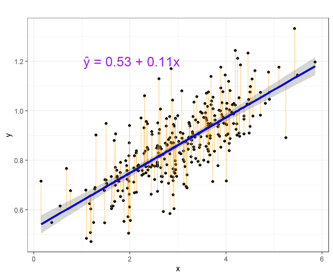
This plot visualizes a simple linear regression. The blue line is the fitted model, with its equation shown. The black dots are the observed data points, and the vertical orange lines represent the residuals—the error between the observed values and the values predicted by the model.

Fitting a Linear Model in R

Fitting a linear model in R is remarkably straightforward using the lm() function, which stands for "linear model". The primary arguments are a formula and a data frame. The formula uses a special syntax, outcome ~ predictor, where the tilde ~ means "is modeled by".

This video from MarinStatsLectures provides an excellent practical walkthrough of the entire process, from plotting the data to fitting the model and interpreting the initial results.

Simple Linear Regression in R | R Tutorial 5.1 | MarinStatsLectures

This video covers the essential R commands for running and summarizing a simple linear regression.

Please watch the following segments: Initial exploration: This shows how to create a scatter plot and check the correlation, which should always be your first step. Fitting the model: Pay close attention to the lm() command and the outcome ~ predictor formula. Interpreting the summary: This segment provides a concise overview of the rich output from the summary() function, which we will dissect in the next section.

Interpreting the Model Output

Once you've fit a model object, like mod <- lm(lung_capacity ~ age, data = my_data), the real work of interpretation begins. The summary() function is your primary tool for this. Its output can seem dense at first, but each piece tells an important part of the story.

To help build your intuition for this, the next video from StatQuest provides a clear, step-by-step explanation of each section of the summary() output.

Linear Regression in R, Step-by-Step

Josh Starmer breaks down the summary() output of a linear model, explaining what each value means conceptually.

Watch from the summary function walkthrough. Focus on his explanations for: Residuals: A quick check on how well the model is balanced around the data. Coefficients: The core of the model, containing the estimates for the intercept and slope, along with their p-values. R-squared: A key measure of how well your model explains the outcome variable.

A Complete Example with Clinical Data

Let's synthesize these concepts with a worked example relevant to your interests in medical research. We will use a dataset containing information on cholesterol levels and blood pressure. The following reading provides all the necessary code and context.

Chapter 7 Linear Regression | Data Analysis in Medicine ...

This chapter from "Data Analysis in Medicine and Health using R" walks through a full simple linear regression analysis, from data exploration to final interpretation.

Please read through the following sections: Start with "About Simple Linear Regression" to solidify the definition. In the "Data exploration" section, review the code for examining the variables chol (cholesterol) and dbp (diastolic blood pressure). Next, read the "Univariable analysis" section carefully. This is the heart of the lesson. It shows you how to: Fit the model using lm(chol ~ dbp, data = coronary). View the standard summary() output. Use broom::tidy() to get a clean data frame of the results, which is a workflow you're already familiar with. Finally, read the "Presentation and interpretation" section. This shows how to construct the model equation and translate the statistical output into a clear, meaningful conclusion.

Let's summarize the key interpretation points from that reading:

Model Equation: From the tidy() output, the intercept estimate is 3.00 and the dbp estimate (the slope) is 0.0389. This gives us the equation:
$chol = 3.00 + 0.0389 \times dbp$
Interpretation of Coefficients:
- Intercept ( $β_{0} = 3.00$ ): A patient with a diastolic blood pressure of 0 mmHg is predicted to have a cholesterol level of 3.00 mmol/L. Clinically, this is an extrapolation far outside the range of the data and is not meaningful on its own. The intercept is primarily a mathematical anchor for the line.
- Slope ( $β_{1} = 0.0389$ ): For every 1 mmHg increase in diastolic blood pressure, the model predicts a 0.0389 mmol/L increase in cholesterol level. This is the key insight.
Statistical Significance: The p-value for the dbp predictor is extremely small (3.92e-10), far below the conventional threshold of 0.05. This tells us that the association between diastolic blood pressure and cholesterol is statistically significant.
Model Fit (R-squared): The summary output shows an R-squared of 0.1798. This means that approximately 18% of the variation in cholesterol levels in this dataset can be explained by the variation in diastolic blood pressure. The other 82% is explained by other factors not included in this simple model.

This is another example from a different analysis, predicting weight from height. The highlighted coefficient, 106.5, is the slope ($\beta_1$). It means that for every 1-meter increase in height, weight is predicted to increase by 106.5 kg. The R-Sq (R-squared) of 49.7% indicates that height explains about half the variability in weight in this sample.

A Note on Categorical Predictors

Simple linear regression isn't limited to numeric predictors. It can also handle a single categorical predictor, and in doing so, it becomes mathematically equivalent to a two-sample t-test. This is extremely useful in clinical research for comparing two groups, like a treatment and a control.

Chapter 6 Linear regression with R | Introduction to Bio-Medical data ...

This section explains how lm() handles categorical predictors by creating "dummy variables" and how to interpret the resulting coefficients.

Read the example under the heading "Example simple...". Focus on the model lm(charges ~ smoker, data=dlm). Notice how R automatically treats the "no" category as the baseline. The intercept becomes the average charge for non-smokers, and the smokeryes coefficient represents the additional average charge for smokers compared to non-smokers.

Conclusion

In this lesson, you've taken a significant step into the world of statistical modeling. You've moved beyond simply testing for associations to quantifying and describing them with a predictive equation.

Key Takeaways:

Simple linear regression models the linear relationship between one outcome and one predictor using the equation $y^= β_{0} + β_{1} x$ .
The lm() function in R is used to fit these models with the outcome ~ predictor formula.
The summary() and broom::tidy() functions are used to extract and interpret model results.
The intercept ( $β_{0}$ ) is the predicted outcome when the predictor is zero.
The slope ( $β_{1}$ ) is the predicted change in the outcome for a one-unit increase in the predictor. Its p-value tells you if the association is statistically significant.
R-squared measures the proportion of variance in the outcome that is explained by the predictor.

Preview of the Next Lesson:
Fitting a model is just the first step. A model is only useful if its underlying assumptions are met. How do we know if a straight line was actually the right choice? In our next lesson, you will learn how to assess linear regression assumptions using diagnostic plots to determine if your model is a reliable and valid representation of the data.